> For the complete documentation index, see [llms.txt](https://kmis.gitbook.io/statistics/llms.txt). Markdown versions of documentation pages are available by appending `.md` to page URLs; this page is available as [Markdown](https://kmis.gitbook.io/statistics/chapter-7.-estimation/7-2.-small-sample-estimation-of-a-population-mean.md).
# 7-2. Small Sample Estimation of a Population Mean
The confidence interval formulas in the previous section are based on the Central Limit Theorem, the statement that for large samples $$\bar{X}$$ is normally distributed with mean $$μ$$ and standard deviation $$σ/\sqrt{n}$$ . When the population mean $$μ$$ is estimated with a small sample ( $$n < 30$$ ), the Central Limit Theorem does not apply. In order to proceed we assume that the numerical population from which the sample is taken has a normal distribution to begin with. If this condition is satisfied then when the population standard deviation *σ* is known the old formula $$\bar{x}±z\_{α∕2}(σ/\sqrt{n})$$ can still be used to construct a $$100(1−α)%$$ confidence interval for $$μ$$ .
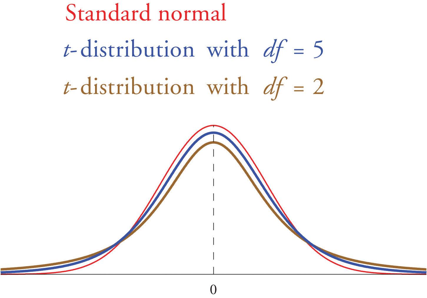
If the population standard deviation is unknown and the sample size *n* is small then when we substitute the sample standard deviation *s* for *σ* the normal approximation is no longer valid. The solution is to use a different distribution, called Student’s *t*-distribution **with** $$(n−1)$$ degrees of freedom. Student’s *t*-distribution is very much like the standard normal distribution in that it is centered at 0 and has the same qualitative bell shape, but it has heavier tails than the standard normal distribution does, as indicated by Figure "Student’s ", in which the curve (in brown) that meets the dashed vertical line at the lowest point is the *t*-distribution with two degrees of freedom, the next curve (in blue) is the *t*-distribution with five degrees of freedom, and the thin curve (in red) is the standard normal distribution. As also indicated by the figure, as the sample size $$n$$ increases, Student’s *t*-distribution ever more closely resembles the standard normal distribution. Although there is a different *t*-distribution for every value of $$n$$ , once the sample size is 30 or more it is typically acceptable to use the standard normal distribution instead, as we will always do in this text.
Just as the symbol $$z\_c$$ stands for the value that cuts off a right tail of area $$c$$ in the standard normal distribution, so the symbol $$t\_c$$ stands for the value that cuts off a right tail of area $$c$$ in the standard normal distribution. This gives us the following confidence interval formulas.
> **Small Sample** $$100(1−α)%$$ **Confidence Interval for a Population Mean**
>
> If $$σ$$ is known: $$\bar{x}±z\_{α∕2}(σ/\sqrt{n})$$
>
> If $$σ$$ is unknown: $$\bar{x}±t\_{α∕2}(s/\sqrt{n})$$ (degrees of freedom $$df=(n−1)$$ )
>
> The population must be normally distributed.
>
> A sample is considered small when $$n < 30$$ .
To use the new formula we use the line in [Figure 12.3 "Critical Values of "](https://saylordotorg.github.io/text_introductory-statistics/s16-appendix.html) that corresponds to the relevant sample size.
**EXAMPLE 5.** **A sample of size 15** drawn from a normally distributed population has sample mean 35 and sample standard deviation 14. Construct a 95% confidence interval for the population mean, and interpret its meaning.
**\[ Solution ]**
Since the population is normally distributed, the sample is small, and the population standard deviation is unknown, the formula that applies is $$\bar{x} ±t\_{α∕2} \frac {s} { \sqrt{n}}$$.
Confidence level 95% means that $$α=1−0.95=0.05$$ so $$α∕2=0.025$$ . Since the sample size is $$n = 15$$ , there are $$n−1=14$$ degrees of freedom. By Figure 12.3 "Critical Values of " $$t\_{0.025} =2.145$$ . Thus $$\bar{x} ± t\_{α∕2} \frac {s} { \sqrt{n}} = 35 ± 2.145 ( \frac {14}{\sqrt {15} } )=35±7.8$$ .
One may be 95% confident that the true value of $$μ$$ is contained in the interval $$(35−7.8,35+7.8)=(27.2,42.8)$$ .
{% tabs %}
{% tab title="R Source" %}
```
n <- 15
mu <- 35
sd <- 14
alpha <- 0.05
se <- sd / sqrt(n)
t <- qt(1-alpha/2, n-1); t
ll <- mu - t * se
ul <- mu + t * se
ll # lower limit
ul # upper limit
```
{% endtab %}
{% tab title="Result" %}
```
> t <- qt(1-alpha/2, n-1); t
## [1] 2.144787
>
> ll <- mu - t * se
> ul <- mu + t * se
> ll # lower limit
## [1] 27.24706
> ul # upper limit
## [1] 42.75294
```
{% endtab %}
{% endtabs %}
* Using **Rstat** Package : `pmean.ci2()`
{% tabs %}
{% tab title="R Source" %}
```
library(Rstat)
pmean.ci2(xb=35, sig=14, n=15, alp=0.05, dig=3)
```
{% endtab %}
{% tab title="Result" %}
```
> pmean.ci2(xb=35, sig=14, n=15, alp=0.05, dig=3)
## [35 ± 2.145×14/√15] = [35 ± 7.753] = [27.247, 42.7]
```
{% endtab %}
{% endtabs %}
**EXAMPLE 6.** A random **sample of 12 students** from a large university yields mean GPA 2.71 with sample standard deviation 0.51. Construct a 90% confidence interval for the mean GPA of all students at the university. Assume that the numerical population of GPAs from which the sample is taken has a normal distribution.
**\[ Solution ]**
Since the population is normally distributed, the sample is small, and the population standard deviation is unknown, the formula that applies is $$\bar{x} ±t\_{α∕2} \frac {s} { \sqrt{n}}$$ .
Confidence level 95% means that $$α=1−0.90=0.10$$ so $$α∕2=0.05$$. Since the sample size is $$n = 12$$ , there are $$n−1=11$$ degrees of freedom. By Figure 12.3 "Critical Values of " $$t\_{0.05} =1.796$$ . Thus $$\bar{x} ± t\_{α∕2} \frac {s} { \sqrt{n}} = 2.71 ± 1.796 ( \frac {0.51}{\sqrt {12} } )=2.71±0.26$$ .
One may be 95% confident that the true value of $$μ$$ is contained in the interval $$(2.71−0.26, 2.71+0.26)=(2.45,2.97)$$.
{% tabs %}
{% tab title="R Source" %}
```
n <- 12
mu <- 2.71
sd <- 0.51
alpha <- 0.10
se <- sd / sqrt(n)
t <- qt(1-alpha/2, n-1); t
ll <- mu - t * se
ul <- mu + t * se
ll # lower limit
ul # upper limit
```
{% endtab %}
{% tab title="Result" %}
```
> t <- qt(1-alpha/2, n-1); t
## [1] 1.795885
>
> ll <- mu - t * se
> ul <- mu + t * se
> ll # lower limit
## [1] 2.445602
> ul # upper limit
## [1] 2.974398
```
{% endtab %}
{% endtabs %}
* Using **Rstat** Package : `pmean.ci2()`
{% tabs %}
{% tab title="R Source" %}
```
library(Rstat)
pmean.ci2(xb=2.71, sig=0.51, n=12, alp=0.10, dig=3)
```
{% endtab %}
{% tab title="Result" %}
```
> pmean.ci2(xb=2.71, sig=0.51, n=12, alp=0.10, dig=3)
## [2.71 ± 1.796×0.51/√12] = [2.71 ± 0.264] = [2.446, 2.974]
```
{% endtab %}
{% endtabs %}
---
# Agent Instructions
This documentation is published with GitBook. GitBook is the documentation platform designed so that both humans and AI agents can read, navigate, and reason over technical content effectively. Learn more at gitbook.com.
## Querying This Documentation
If you need additional information that is not directly available in this page, you can query the documentation dynamically by asking a question.
Perform an HTTP GET request on the current page URL with the `ask` query parameter, and the optional `goal` query parameter:
```
GET https://kmis.gitbook.io/statistics/chapter-7.-estimation/7-2.-small-sample-estimation-of-a-population-mean.md?ask=&goal=
```
`ask` is the immediate question: it should be specific, self-contained, and written in natural language.
`goal` is optional and describes the broader end goal you are ultimately trying to accomplish on behalf of the user. GitBook uses it to tailor the answer towards what is most useful for that goal.
The response will contain a direct answer to the question and relevant excerpts and sources from the documentation.
Use this mechanism when the answer is not explicitly present in the current page, you need clarification or additional context, or you want to retrieve related documentation sections.