10-4. The Least Squares Regression Line

1. Goodness of Fit of a Straight Line to Data

Once the scatter diagram of the data has been drawn and the model assumptions described in the previous sections at least visually verified (and perhaps the correlation coefficient $r$ computed to quantitatively verify the linear trend), the next step in the analysis is to find the straight line that best fits the data. We will explain how to measure how well a straight line fits a collection of points by examining how well the line $y=\frac{1}{2}x−1$ fits the data set

x 2 2 6 8 10 y 0 1 2 3 3

(which will be used as a running example for the next three sections). We will write the equation of this line as $\hat{y}=\frac{1}{2}x−1$ with an accent on the $y$ to indicate that the $y$-values computed using this equation are not from the data. We will do this with all lines approximating data sets. The line $\hat{y}=\frac{1}{2}x−1$ was selected as one that seems to fit the data reasonably well.

The idea for measuring the goodness of fit of a straight line to data is illustrated in Figure 10.6 "Plot of the Five-Point Data and the Line ", in which the graph of the line $\hat{y}=\frac{1}{2}x−1$ has been superimposed on the scatter plot for the sample data set.

Figure 10.6 Plot of the Five-Point Data and the Line $\hat{y}=\frac{1}{2}x−1$

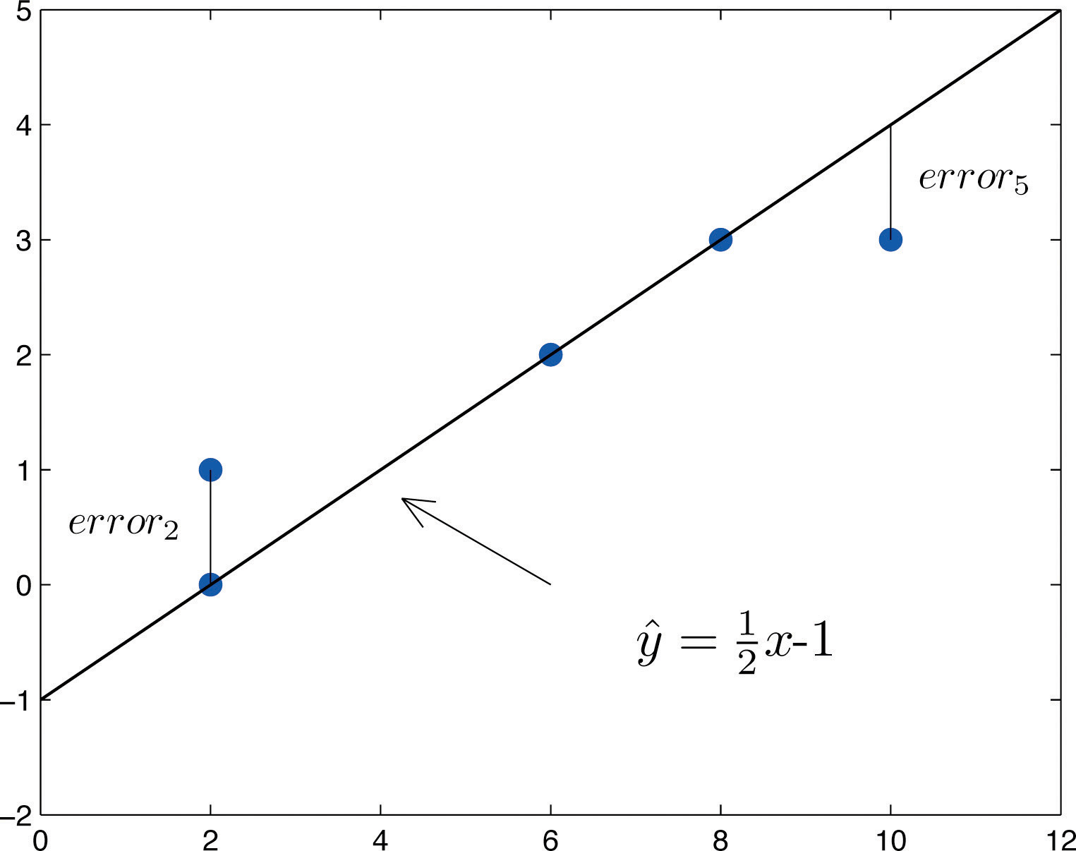
To each point in the data set there is associated an “error,” the positive or negative vertical distance from the point to the line: positive if the point is above the line and negative if it is below the line.

The error can be computed as the actual $y$-value of the point minus the $y$-value $\hat{y}$ that is “predicted” by inserting the x-value of the data point into the formula for the line:

$error at data point (x,y)=(true y)−(predicted y)=y− \hat{y}$

The computation of the error for each of the five points in the data set is shown in Table 10.1 "The Errors in Fitting Data with a Straight Line".

Table 10.1 The Errors in Fitting Data with a Straight Line

	$x$	$y$	$\hat{y}=\frac{1}{2}x−1$	$y− \hat{y}$	$(y− \hat{y})^2$
	2	0	0	0	0
	2	1	0	1	1
	6	2	2	0	0
	8	3	3	0	0
	10	3	4	−1	1
$Σ$	-	-	-	0	2

A first thought for a measure of the goodness of fit of the line to the data would be simply to add the errors at every point, but the example shows that this cannot work well in general. The line does not fit the data perfectly (no line can), yet because of cancellation of positive and negative errors the sum of the errors (the fourth column of numbers) is zero.

Instead goodness of fit is measured by the sum of the squares of the errors. Squaring eliminates the minus signs, so no cancellation can occur. For the data and line in Figure 10.6 "Plot of the Five-Point Data and the Line " the sum of the squared errors (the last column of numbers) is 2. This number measures the goodness of fit of the line to the data.

The goodness of fit of a line $\hat{y}=mx + b$ to a set of $n$ pairs $(x,y)$ of numbers in a sample is the sum of the squared errors

$Σ(y−\hat{y})^2$

( $n$ terms in the sum, one for each data pair).

2. The Least Squares Regression Line

Given any collection of pairs of numbers (except when all the $x$ -values are the same) and the corresponding scatter diagram, there always exists exactly one straight line that fits the data better than any other, in the sense of minimizing the sum of the squared errors. It is called the least squares regression line. Moreover there are formulas for its slope and y-intercept.

Given a collection of pairs $(x,y)$ of numbers (in which not all the x-values are the same), there is a line $\hat{y}=\hat{β_1}x+\hat{β_0}$ that best fits the data in the sense of minimizing the sum of the squared errors. It is called the least squares regression line. Its slope $\hat{β_1}$ and $y$ -intercept $\hat{β_0}$ are computed using the formulas

$\hat{β_1}= \frac{SS_{xy}} {SS_{xx}}$  and  $\hat{β_0} =\bar{y}−\hat{β_1} \bar{x}$

where $SS_{xx}=Σx^2− \frac{1}{n}(Σx)^2$ ,  $SS_{xy}=Σxy− \frac{1}{n}(Σx)(Σy)$

$\bar{x}$ is the mean of all the $x$ -values, $\bar{y}$ is the mean of all the $y$ -values, and $n$ is the number of pairs in the data set.

The equation $\hat{y}=\hat{β_1}x+\hat{β_0}$ specifying the least squares regression line is called the least squares regression equation.

Remember from Section 10.3 "Modelling Linear Relationships with Randomness Present" that the line with the equation $\hat{y}=\hat{β_1}x+\hat{β_0}$ is called the population regression line. The numbers $\hat{β_1}$ and $\hat{β_0}$ are statistics that estimate the population parameters ${β_1}$ and ${β_0}$.

We will compute the least squares regression line for the five-point data set, then for a more practical example that will be another running example for the introduction of new concepts in this and the next three sections.

EXAMPLE 2. Find the least squares regression line for the five-point data set

x 2 2 6 8 10 y 0 1 2 3 3

and verify that it fits the data better than the line $\hat{y}=\frac{1}{2}x−1$ considered in Section 10.4.1 "Goodness of Fit of a Straight Line to Data".

[ Solution ]

$SS_{xx}=Σx^2− \frac{1}{n}(Σx)^2 = 208− \frac{(28)^2} {5}=51.2$

$SS_{xy}=Σxy− \frac{1}{n}(Σx)(Σy) = 68- \frac{(28)(9)}{5} = 17.6$

$\bar{x} = \frac{Σ​x}{n}= \frac{28}{5}=5.6$

$\bar{y} = \frac{Σ​y}{n}= \frac{9}{5}=1.8$

so that

$\hat{β_1}= \frac{SS_{xy}} {SS_{xx}} = \frac{17.6}{51.2}=0.34375$

$\hat{β_0} =\bar{y}−\hat{β_1} \bar{x} =1.8−(0.34375)(5.6)=−0.125$

The least squares regression line for these data is

$\hat{y}=0.34375 x−0.125$

The computations for measuring how well it fits the sample data are given in Table 10.2 "The Errors in Fitting Data with the Least Squares Regression Line". The sum of the squared errors is the sum of the numbers in the last column, which is 0.75. It is less than 2, the sum of the squared errors for the fit of the line $\hat{y}=\frac{1}{2} x−1$ to this data set.

TABLE 10.2 THE ERRORS IN FITTING DATA WITH THE LEAST SQUARES REGRESSION LINE

$x$	$y$	$\hat{y}=0.34375 x−0.125$	$y− \hat{y}$	$(y− \hat{y})^2$
2	0	0.5625	−0.5625	0.31640625
2	1	0.5625	0.4375	0.19140625
6	2	1.9375	0.0625	0.00390625
8	3	2.6250	0.3750	0.14062500
10	3	3.3125	−0.3125	0.09765625

R Source

library(Rstat)

x <- c(2, 2, 6, 8, 10)
y <- c(0, 1, 2, 3, 3)

plot(x, y)
abline(lm(y~x))

corr.reg1(x, y, step=7)

Scatter Diagram

Regression Equation

> corr.reg1(x, y, step=7)
## [Step 7] Estimate simple regression coefficients ------------------
## Sxx = 208 - (28)²/ 5 = 51.2 
## Sxy = 68 - (28 × 9) / 5 = 17.6 
## Slope = 17.6 / 51.2 = 0.3438 
## Intersection = 1.8 - 0.3438 × 5.6 = -0.125 
## Regression Equation : y = -0.125 + 0.3438 x 

EXAMPLE 3. Table 10.3 "Data on Age and Value of Used Automobiles of a Specific Make and Model" shows the age in years and the retail value in thousands of dollars of a random sample of ten automobiles of the same make and model.

1. Construct the scatter diagram.

2. Compute the linear correlation coefficient r. Interpret its value in the context of the problem.

3. Compute the least squares regression line. Plot it on the scatter diagram.

4. Interpret the meaning of the slope of the least squares regression line in the context of the problem.

5. Suppose a four-year-old automobile of this make and model is selected at random. Use the regression equation to predict its retail value.

6. Suppose a 20-year-old automobile of this make and model is selected at random. Use the regression equation to predict its retail value. Interpret the result.

7. Comment on the validity of using the regression equation to predict the price of a brand new automobile of this make and model.

TABLE 10.3 DATA ON AGE AND VALUE OF USED AUTOMOBILES OF A SPECIFIC MAKE AND MODEL

x	2	3	3	3	4	4	5	5	5	6
y	28.7	24.8	26.0	30.5	23.8	24.6	23.8	20.4	21.6	22.1

[ Solution ]

Figure 10.7 Scatter Diagram for Age and Value of Used Automobiles

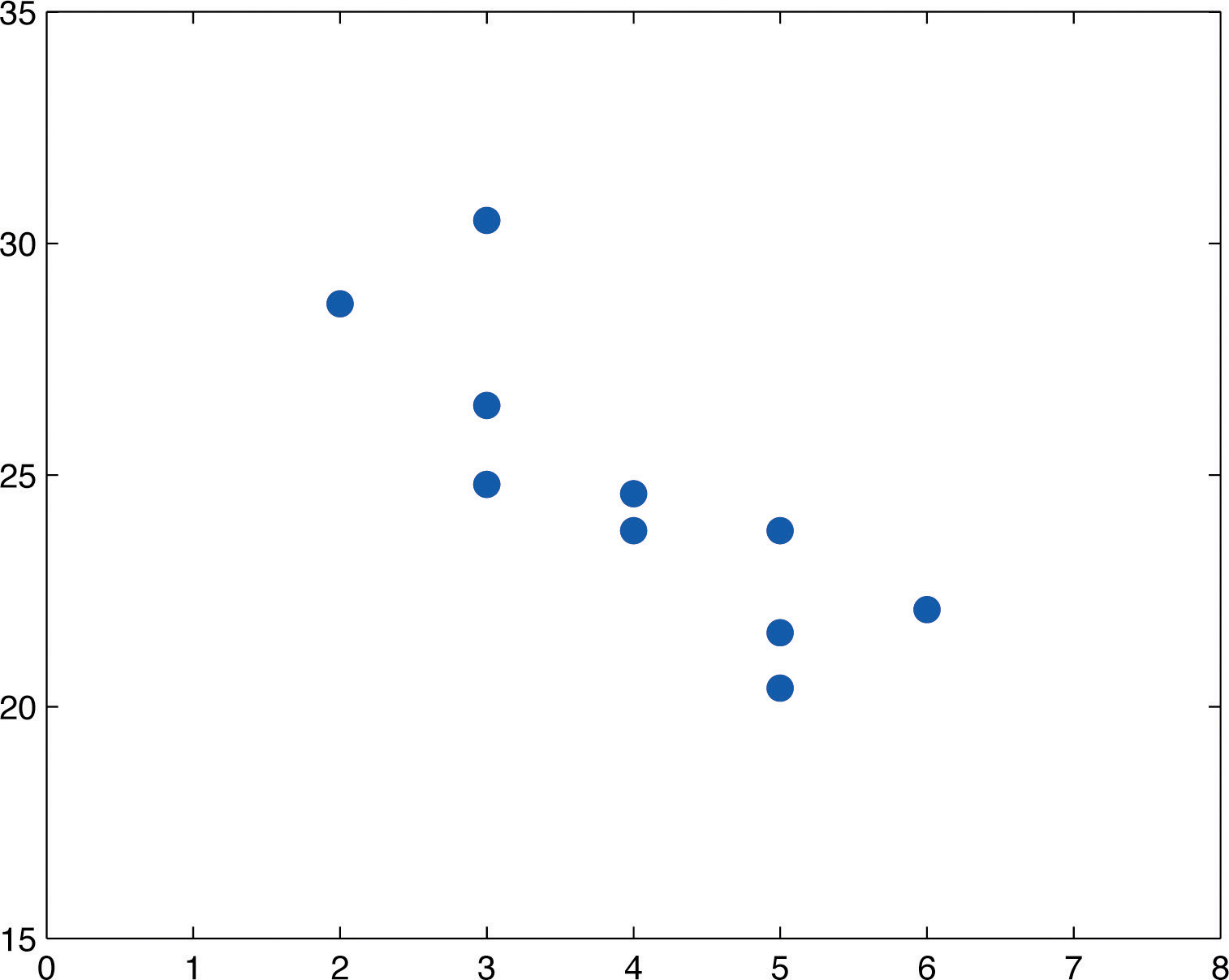
1. The scatter diagram is shown in Figure 10.7 "Scatter Diagram for Age and Value of Used Automobiles".

2. We must first compute $SS_{xx}, SS_{xy}, SS_{yy},$ which means computing $Σx$ , $Σy$ , $Σx^2$ , $Σy^2$, and $Σxy$. Using a computing device we obtain $Σ​x=40, Σ​y=246.3, Σ​x^2=174, Σ​y^2=6154.15, Σ​xy=956.5$ Thus $SS_{xx}=Σx^2− \frac{1}{n}(Σx)^2 = 174− \frac{(40)^2} {10}=14$

   $SS_{xy}=Σxy− \frac{1}{n}(Σx)(Σy) = 956.5- \frac{(40)(246.3)}{10} = -28.7$ $SS_{yy}=Σy^2− \frac{1}{n}(Σy)^2 = 6154.15− \frac{(246.3)^2} {10}=87.781$

   so that

   $r= \frac{SS_{xy}} {\sqrt{SS_{xx}⋅SS_{yy}}}= \frac{(-28.7) } {\sqrt{ (14)(87.781)}} = -0.819$ The age and value of this make and model automobile are moderately strongly negatively correlated. As the age increases, the value of the automobile tends to decrease.

3. Using the values of $Σx$ and $Σy$ computed in part (b), $\bar{x} = \frac{Σ​x}{n}= \frac{40}{10}=4$

   $\bar{y} = \frac{Σ​y}{n}= \frac{246.3}{10}=24.63$

   Thus using the values of $SS_{xx} and \space SS_{xy}$ from part (b), $\hat{β_1}= \frac{SS_{xy}} {SS_{xx}} = \frac{-28.7}{14}=-2.05$

   $\hat{β_0} =\bar{y}−\hat{β_1} \bar{x} =24.63−(-2.05)(4)=32.83$

   The equation $\hat{y}=\hat{β_1}x+\hat{β_0}$ of the least squares regression line for these sample data is

   $\hat{y}=-2.05 x + 32.83$ Figure 10.8 "Scatter Diagram and Regression Line for Age and Value of Used Automobiles" shows the scatter diagram with the graph of the least squares regression line superimposed. Figure 10.8 Scatter Diagram and Regression Line for Age and Value of Used Automobiles

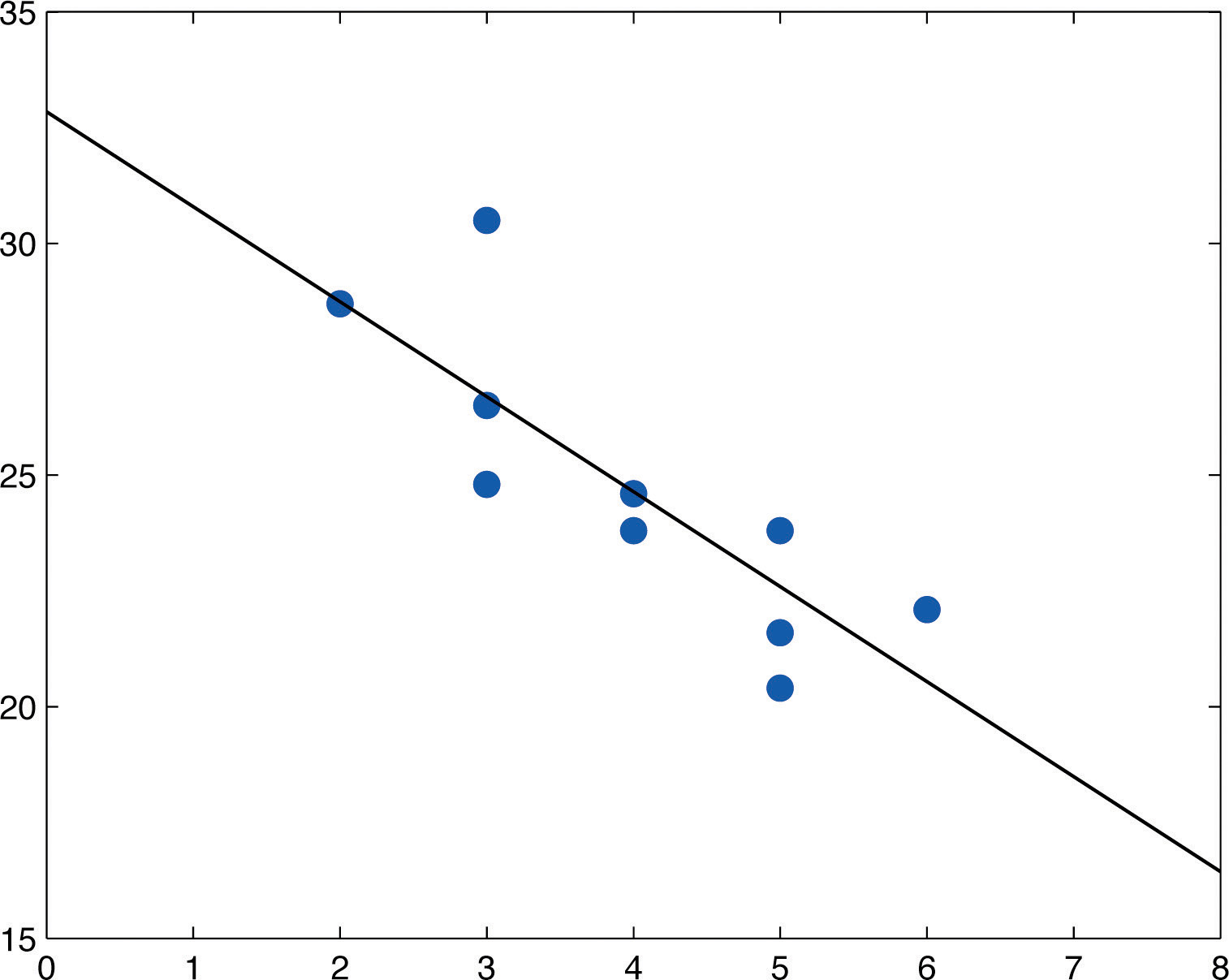
1. The slope −2.05 means that for each unit increase in $x$ (additional year of age) the average value of this make and model vehicle decreases by about 2.05 units (about $2,050).

2. Since we know nothing about the automobile other than its age, we assume that it is of about average value and use the average value of all four-year-old vehicles of this make and model as our estimate. The average value is simply the value of $\hat{y}$ obtained when the number 4 is inserted for $x$ in the least squares regression equation:

   $\hat{y}=-2.05 x + 32.83 = -2.05 (4) + 32.83 = 24.63$

   which corresponds to $24,630.

3. Now we insert $x=20$ into the least squares regression equation, to obtain

   $\hat{y}=-2.05 x + 32.83 = -2.05 (20) + 32.83 = -8.17$

   which corresponds to −$8,170. Something is wrong here, since a negative makes no sense. The error arose from applying the regression equation to a value of $x$ not in the range of $x$ -values in the original data, from two to six years.

   Applying the regression equation $\hat{y}=\hat{β_1}x+\hat{β_0}$ to a value of $x$ outside the range of $x$ -values in the data set is called extrapolation. It is an invalid use of the regression equation and should be avoided.

4. The price of a brand new vehicle of this make and model is the value of the automobile at age 0. If the value $x=0$ is inserted into the regression equation the result is always $\hat{β_0}$ , the $y$ -intercept, in this case 32.83, which corresponds to $32,830. But this is a case of extrapolation, just as part (f) was, hence this result is invalid, although not obviously so. In the context of the problem, since automobiles tend to lose value much more quickly immediately after they are purchased than they do after they are several years old, the number $32,830 is probably an underestimate of the price of a new automobile of this make and model.

R Source

library(Rstat)

x <- c(2, 3, 3, 3, 4, 4, 5, 5, 5, 6)
y <- c(28.7, 24.8, 26.0, 30.5, 23.8, 24.6, 23.8, 20.4, 21.6, 22.1)

plot(x, y)
abline(lm(y~x))

corr.reg1(x, y, step=7)

Scatter Diagram

Regression Equation

> corr.reg1(x, y, step=7)
## [Step 7] Estimate simple regression coefficients ------------------
## Sxx = 174 - (40)²/ 10 = 14 
## Sxy = 956.5 - (40 × 246.3) / 10 = -28.7 
## Slope = -28.7 / 14 = -2.05 
## Intersection = 24.63 - -2.05 × 4 = 32.83 
## Regression Equation : y = 32.83 - 2.05 x 
##

For emphasis we highlight the points raised by parts (f) and (g) of the example.

The process of using the least squares regression equation to estimate the value of y at a value of x that does not lie in the range of the x-values in the data set that was used to form the regression line is called extrapolation. It is an invalid use of the regression equation that can lead to errors, hence should be avoided.

3. The Sum of the Squared Errors $(SSE)$

In general, in order to measure the goodness of fit of a line to a set of data, we must compute the predicted y-value yˆy^ at every point in the data set, compute each error, square it, and then add up all the squares. In the case of the least squares regression line, however, the line that best fits the data, the sum of the squared errors can be computed directly from the data using the following formula.

The sum of the squared errors for the least squares regression line is denoted by SSE.SSE. It can be computed using the formula

$SSE=SS_{yy}−\hat{β_1}SS_{xy}$

EXAMPLE 4. Find the sum of the squared errors $SSE$ for the least squares regression line for the five-point data set

x 2 2 6 8 10 y 0 1 2 3 3

Do so in two ways:

1. using the definition $Σ(y−\hat{y})^2$ ;

2. using the formula $SSE=SS_{yy}−\hat{β_1}SS_{xy}$.

   .

[ Solution ]

1. The least squares regression line was computed in Note 10.18 "Example 2" and is $\hat{y}=0.34375 x−0.125$. $SSE$ was found at the end of that example using the definition $Σ(y−\hat{y})^2$. The computations were tabulated in Table 10.2 "The Errors in Fitting Data with the Least Squares Regression Line". $SSE$ is the sum of the numbers in the last column, which is 0.75.

2. The numbers $SS_{xy}$ and $\hat{β_1}$ were already computed in Note 10.18 "Example 2" in the process of finding the least squares regression line. So was the number $Σy=9$ . We must compute $SS_{yy}$. To do so it is necessary to first compute $Σy^2=0+1^2+2^2+3^2+3^2=23$ Then

   $SS_{yy}=Σy^2− \frac{1}{n}(Σy)^2 = 23− \frac{(9)^2} {5}=6.8$ so that $SSE=SS_{yy}−\hat{β_1}SS_{xy} = 6.8 - (0.34375)(17.6) = 0.75$

EXAMPLE 5. Find the sum of the squared errors $SSE$ for the least squares regression line for the data set, presented in Table 10.3 "Data on Age and Value of Used Automobiles of a Specific Make and Model", on age and values of used vehicles in Note 10.19 "Example 3".

[ Solution ]

From Note 10.19 "Example 3" we already know that $SS_{xy}=−28.7$ ,  $\hat{β_1}=−2.05$ , and  $Σy=246.3$ .

To compute $SS_{yy}$ we first compute

$Σy^2=28.7^2+24.8^2+26.0^2+30.5^2+23.8^2+24.6^2+23.8^2+20.4^2$ $+21.6^2+22.1^2=6154.15$

Then

$SS_{yy}=Σy^2− \frac{1}{n}(Σy)^2 = 6154 -\frac{(246.3)^2} {10} = 87.781$

Therefore

$SSE=SS_{yy}−\hat{β_1}SS_{xy} = 87.781 - (-2.05)(-28.7) = 28.946$.