10-2. The Linear Correlation Coefficient

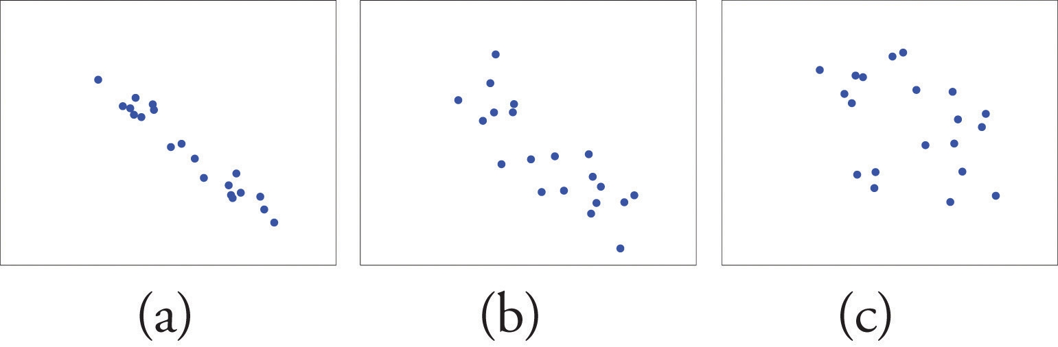
Figure 10.3 "Linear Relationships of Varying Strengths" illustrates linear relationships between two variables $x$ and $y$ of varying strengths. It is visually apparent that in the situation in panel (a), $x$ could serve as a useful predictor of $y$ , it would be less useful in the situation illustrated in panel (b), and in the situation of panel (c) the linear relationship is so weak as to be practically nonexistent. The linear correlation coefficient is a number computed directly from the data that measures the strength of the linear relationship between the two variables $x$ and $y$.

Figure 10.3 Linear Relationships of Varying Strengths

The linear correlation coefficient for a collection of $n$ pairs $(x,y)$ of numbers in a sample is the number $r$ given by the formula

$r= \frac{SS_{xy}} {\sqrt{SS_{xx}⋅SS_{yy}}}$

where $SS_{xx}=Σx^2− \frac{1}{n}(Σx)^2$ ,  $SS_{xy}=Σxy− \frac{1}{n}(Σx)(Σy)$ ,   $SS_{yy}=Σy^2− \frac{1}{n}(Σy)^2$

The linear correlation coefficient has the following properties, illustrated in Figure 10.4 "Linear Correlation Coefficient ":

1. The value of $r$ lies between −1 and 1, inclusive.

2. The sign of $r$ indicates the direction of the linear relationship between $x$ and $y$:

   1. If $r<0$ then $y$ tends to decrease as $x$ is increased.

   2. If $r>0$ then $y$tends to increase as $x$ is increased.

3. The size of $|r|$ indicates the strength of the linear relationship between $x$ and $y$:

   1. If $|r|$ is near 1 (that is, if $r$ is near either 1 or −1) then the linear relationship between $x$ and $y$ is strong.

   2. If $|r|$ is near 0 (that is, if $r$ is near 0 and of either sign) then the linear relationship between $x$ and $y$ is weak.

Figure 10.4 Linear Correlation Coefficient R

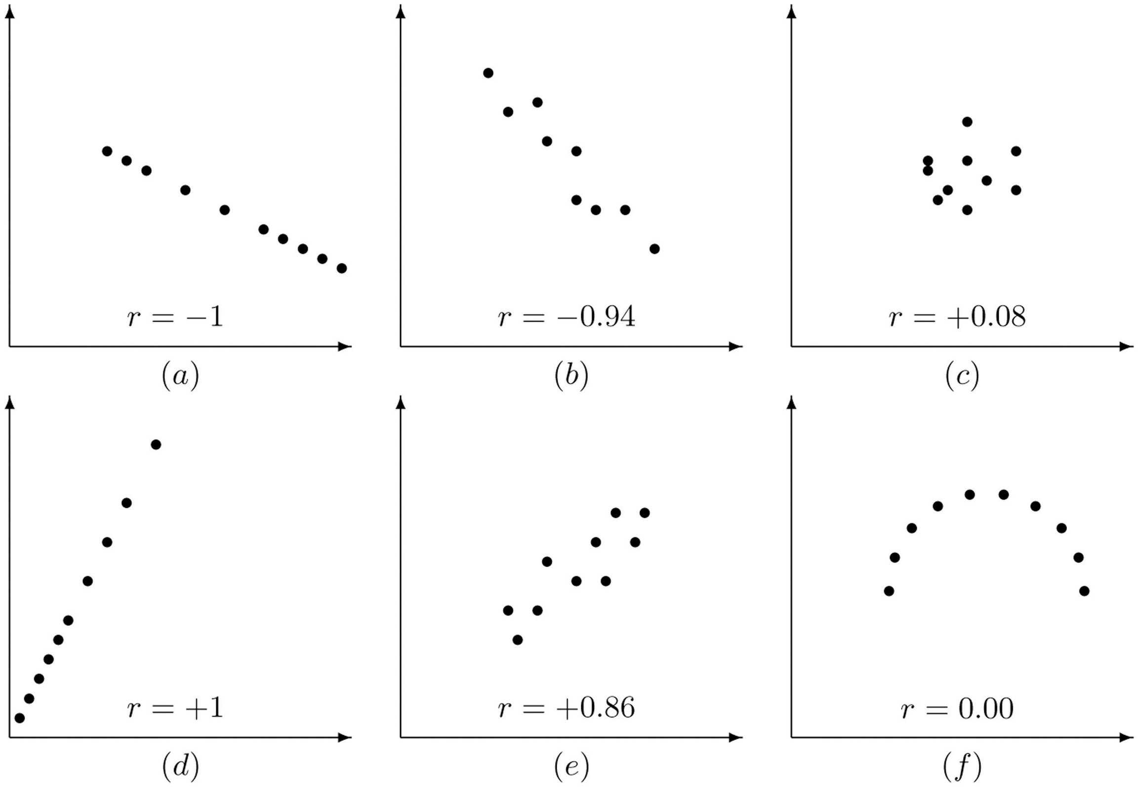
Pay particular attention to panel (f) in Figure 10.4 "Linear Correlation Coefficient ". It shows a perfectly deterministic relationship between $x$ and $y$, but $r=0$ because the relationship is not linear. (In this particular case the points lie on the top half of a circle.)

EXAMPLE 1. Compute the linear correlation coefficient for the height and weight pairs plotted in Figure 10.2 "Plot of Height and Weight Pairs".

[ Solution ]

Even for small data sets like this one computations are too long to do completely by hand. In actual practice the data are entered into a calculator or computer and a statistics program is used. In order to clarify the meaning of the formulas we will display the data and related quantities in tabular form. For each $(x,y)$ pair we compute three numbers: $x^2$ , $xy$ , and $y^2$ , as shown in the table provided. In the last line of the table we have the sum of the numbers in each column. Using them we compute:

362B

ex_10-2.csv

$SS_{xx}=Σx^2− \frac{1}{n}(Σx)^2 = 61537 - \frac{859^2}{12} = 46.916$

$SS_{xy}=Σxy− \frac{1}{n}(Σx)(Σy) = 143626− \frac{(859)(2003)}{12}=244.583$

$SS_{yy}=Σy^2− \frac{1}{n}(Σy)^2 = 336025− \frac{(2003)^2}{12}=1690.916$

so that

$r= \frac{SS_{xy}} {\sqrt{SS_{xx}⋅SS_{yy}}} = \frac{244.583 } {\sqrt {(46.916)(1690.916)}} = 0.868$

The number $r=0.868$ quantifies what is visually apparent from Figure 10.2 "Plot of Height and Weight Pairs": weights tends to increase linearly with height ( $r$ is positive) and although the relationship is not perfect, it is reasonably strong ($r$ is near 1).

R Source

x <- c(68, 69, 70, 70, 71, 72, 72, 72, 73, 73, 74, 75)
y <- c(151, 146, 157, 164, 171, 160, 163, 180, 170, 175, 178, 188)

cor(x, y, method="pearson")

r

> cor(x, y, method="pearson")
## [1] 0.8683647