> For the complete documentation index, see [llms.txt](https://kmis.gitbook.io/statistics/llms.txt). Markdown versions of documentation pages are available by appending `.md` to page URLs; this page is available as [Markdown](https://kmis.gitbook.io/statistics/chapter-4.-discrete-random-variables/4-4.-binomial-distribution.md).
# 4-4. Binomial Distribution
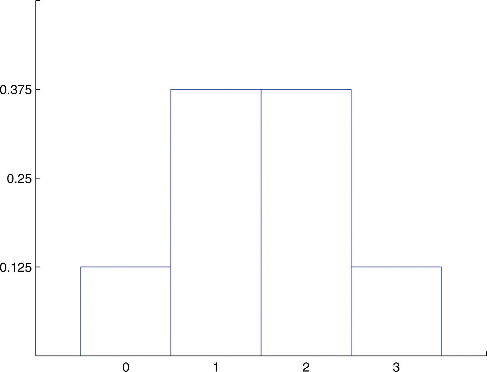
The **experiment** of *tossing a fair coin three times* and **the experiment** of ***observing the genders*** according to birth order of the children in a randomly selected three-child family are **completely different**, but the random variables that count the *number of heads* in the coin toss and the *number of boys* in the family (assuming the two genders are equally likely) are **the same random variable**, the one with probability distribution
| x | 0 | 1 | 2 | 3 |
| ---- | ----- | ----- | ----- | ----- |
| P(x) | 0.125 | 0.375 | 0.375 | 0.125 |
A histogram that graphically illustrates this probability distribution is given in Figure 4.4 "Probability Distribution for Three Coins and Three Children". What is common to the two experiments is that we perform three identical and independent trials of the same action, each trial has only two outcomes (heads or tails, boy or girl), and the probability of success is the same number, 0.5, on every trial.
The random variable that is generated is called the *binomial random variable* **with parameters** $$n = 3$$ **and** $$p = 0.5$$ . This is just one case of a general situation.
Figure 4.4 Probability Distribution for Three Coins and Three Children
> *Suppose a random experiment has the following characteristics.*
>
> 1. *There are* $$n$$ ***identical and independent trials** of a common procedure.*
> 2. *There are **exactly two possible outcomes for each trial,** one termed “**success**” and the other “**failure.**”*
> 3. *The **probability of success** on any one trial is the same number* $$p$$ .
>
> *Then the discrete random variable* $$X$$ *that counts the number of successes in the* $$n$$ *trials is the* ***binomial random variable with parameters*** $$n$$ ***and*** $$p$$ *. We also say that* $$X$$ **has a binomial distribution** **with parameters** *n* **and** *p*.
The following **four examples** illustrate the definition. Note how in every case “success” is the outcome that is counted, not the outcome that we prefer or think is better in some sense.
1. A random sample of 125 students is selected from a large college in which the proportion of students who are females is 57%. Suppose $$X$$ denotes the number of female students in the sample. In this situation there are $$n = 125$$ identical and independent trials of a common procedure, selecting a student at random; there are exactly two possible outcomes for each trial, “success” (what we are counting, that the student be female) and “failure;” and finally the probability of success on any one trial is the same number $$p = 0.57$$ . $$X$$ is a binomial random variable with parameters $$n = 125$$ and $$p = 0.57$$.
2. A multiple-choice test has 15 questions, each of which has five choices. An unprepared student taking the test answers each of the questions completely randomly by choosing an arbitrary answer from the five provided. Suppose $$X$$ denotes the number of answers that the student gets right. $$X$$ is a binomial random variable with parameters $$n = 15$$ and $$p=1∕5=0.20$$ .
3. In a survey of 1,000 registered voters each voter is asked if he intends to vote for a candidate Titania Queen in the upcoming election. Suppose $$X$$ denotes the number of voters in the survey who intend to vote for Titania Queen. $$X$$ is a binomial random variable with $$n = 1000$$ and $$p$$ equal to the true proportion of voters (surveyed or not) who intend to vote for Titania Queen.
4. An experimental medication was given to 30 patients with a certain medical condition. Suppose $$X$$ denotes the number of patients who develop severe side effects. $$X$$ is a binomial random variable with $$n = 30$$ and $$p$$ equal to the true probability that a patient with the underlying condition will experience severe side effects if given that medication.
## 1. Bernoulli Distribution
성공확률( $$p$$ )이 일정한 **1회의 시행**에서 나오는 **성공횟수(** $$X$$ **)의 확률분포(** $$f(X)$$ **)**를 말한다.
> **Bernoulli Distribution**
>
> $$f(x) = p^x(1-p)^{(1-x)},$$ $$x = 0, 1$$
>
> or $$f(x) = \left{\begin{matrix} p, & if \space x=1;\ 1-p, & if \space x=0 \end{matrix}\right.$$
> **Expected Value** and **Variance** of Bernoulli Distribution
>
> $$E(X) = \Sigma xf(x)= 0 \times(1-p) + 1 \times p = p$$
>
> $$Var(X) = E(X^2) - E(X)^2 = p-p^2 = p(1-p)$$
## 2. Probability Formula for a Binomial Random Variable
> If $$X$$ is a binomial random variable with parameters $$n$$ and $$p$$ , then
>
> $$P(X=x) = \frac {n!} {x! (n−x)!} p^x q^{(n−x)}$$ , $$(x = 0, 1, 2 , ..., n)$$
>
> where $$q=(1−p)$$ and where for any counting number $$n$$ , \
> $$n!$$ (read “*n* factorial”) is defined by $$0!=1, 1!=1, 2!=1⋅2, 3!=1⋅2⋅3$$
>
> and in general $$n!=1⋅2 ⋅ ⋅ ⋅ (n−1)⋅n$$
**EXAMPLE 8**. Seventeen percent of victims of financial fraud know the perpetrator of the fraud personally.
1. Use the formula to construct the probability distribution for the number $$X$$ of people in a random sample of five victims of financial fraud who knew the perpetrator personally.
2. A investigator examines five cases of financial fraud every day. Find the most frequent number of cases each day in which the victim knew the perpetrator.
3. A investigator examines five cases of financial fraud every day. Find the average number of cases per day in which the victim knew the perpetrator.
**\[ Solution ]**
1. The random variable $$X$$ is binomial with parameters $$n = 5$$ and $$p = 0.17$$ ; $$q=1−p=0.83.$$ The possible values of $$X$$ are 0, 1, 2, 3, 4, and 5.\
\
$$P(0)= \frac{5!}{0!5!} (0.17)^0 (0.83)^5$$ \
$$=\frac{1⋅2⋅3⋅4⋅5}{(1)⋅(1⋅2⋅3⋅4⋅5)} 1⋅(0.3939040643)$$ \
$$=0.3939040643≈0.3939$$ \
$$P(1)= \frac{5!}{1!4!} (0.17)^1 (0.83)^4$$
$$=\frac{1⋅2⋅3⋅4⋅5}{(1)⋅(1⋅2⋅3⋅4)} (0.17)⋅(0.47458321)$$
$$=0.4033957285≈0.4034$$
$$P(2)= \frac{5!}{2!3!} (0.17)^2 (0.83)^3$$
$$=\frac{1⋅2⋅3⋅4⋅5}{(1,2)⋅(1⋅2⋅3)} (0.289)⋅(0.571787)$$
$$=0.165246443≈0.1652$$
\
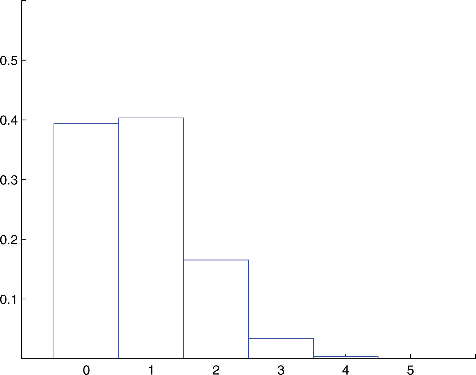
The remaining three probabilities are computed similarly, to give the probability distribution\
\
x 0 1 2 3 4 5\
P(x) 0.3939 0.4034 0.1652 0.0338 0.0035 0.0001\
\
The probabilities do not add up to exactly 1 because of rounding.\
This probability distribution is represented by the histogram in [Figure 4.5 "Probability Distribution of the Binomial Random Variable in "](https://saylordotorg.github.io/text_introductory-statistics/s08-03-the-binomial-distribution.html#fwk-shafer-ch04_s03_s01_f01), which graphically illustrates just how improbable the events $$X=4$$ and $$X=5$$ are. The corresponding bar in the histogram above the number 4 is barely visible, if visible at all, and the bar above 5 is far too short to be visible.\
\
Figure 4.5 Probability Distribution of the Binomial Random Variable in [Note 4.29 "Example 7"](https://saylordotorg.github.io/text_introductory-statistics/s08-03-the-binomial-distribution.html#fwk-shafer-ch04_s03_s01_n02)
1.
2. The value of $$X$$ that is most likely is $$X=1$$, so the most frequent number of cases seen each day in which the victim knew the perpetrator is one.
3. The average number of cases per day in which the victim knew the perpetrator is the mean of $$X$$, which is\
\
$$μ=Σx P(x) = 0⋅0.3939+1⋅0.4034+2⋅0.1652+3⋅0.0338$$ \
$$+ 4⋅0.0035+5⋅0.0001 = 0.8497$$
* Using **Rstat** Package : `dbinom(x, n, p)`and `disc.exp()`
{% tabs %}
{% tab title="R Source" %}
```
library(Rstat)
# 1. Probability Distribution
n <- 5
p <- 0.17
x <- 0:n
px <- dbinom(x, n, p); px
# 2. E(X) and Var(X)
disc.exp(x, px)
# 3. Plot
disc.exp(x, px, prt=FALSE, plot=TRUE)
```
{% endtab %}
{% tab title="E(X) and Var(X)" %}
```
> disc.exp(x, px)
## E(X) = 0.85
## V(X) = 1.428 - 0.85² = 0.706
## D(X) = √(0.706) = 0.84
```
{% endtab %}
{% tab title="Probability Distribution Plot" %}

{% endtab %}
{% endtabs %}
## **2.** Special Formulas for the Mean and Standard Deviation of a Binomial Random Variable
> If $$X$$ is a binomial random variable with parameters $$n$$ and $$p$$ , then
>
> $$E(X) = \Sigma E(X\_i) = \Sigma p=np$$ ($$X\_i :$$$$i ^{th}$$ Bernoulli random variable )
>
> $$Var(X) = \Sigma Var(X\_i) = \Sigma p(1-p) =np(1-p)$$
> \==> $$μ=np$$ , $$σ^2=npq$$, $$σ= \sqrt {npq}$$
>
> where $$q=1-p$$ .
**EXAMPLE 9.** Find the mean and standard deviation of the random variable $$X$$ of "**Example 7**".
**\[ Solution ]**
The random variable *X* is binomial with parameters $$n = 5$$ and $$p = 0.17$$ , and $$q=1−p=0.83$$ . Thus its mean and standard deviation are
$$μ=np=5⋅0.17=0.85 (exactly)$$
and
$$σ=\sqrt{npq}=\sqrt{5⋅0.17⋅0.83}=\sqrt{.7055}≈0.8399$$
## 3. The Cumulative Probability Distribution of a Binomial Random Variable
In the place of the probability $$P(x)$$ the table contains the probability
$$P(X≤x)=P(0)+P(1)+ ⋅ ⋅ ⋅ +P(x)$$
This is illustrated in the followinng Figure "**Cumulative Probabilities**".

> If $$X$$ is a discrete random variable, then
>
> $$P(X≥x)=1−P(X≤x−1)$$
>
> and $$P(x)=P(X≤x)−P(X≤x−1)$$
**EXAMPLE 10.** A student takes a ten-question true/false exam.
1. Find the probability that the student gets exactly six of the questions right simply by guessing the answer on every question.
2. Find the probability that the student will obtain a passing grade of 60% or greater simply by guessing.
**\[ Solution ]**
1. The probability sought is $$P(6)$$ . The formula gives\
$$P(6)=\frac{10!}{(6!)(4!)}(.5)^6(.5)^4=0.205078125$$
Using the table,\
$$P(6)=P(X≤6)−P(X≤5)=0.8281−0.6230=0.2051$$
2. The student must guess correctly on at least 60% of the questions, which is $$(0.60)⋅10=6$$ questions. The probability sought is *not* $$P(6)$$ (an easy mistake to make), but\
$$P(X≥6)=P(6)+P(7)+P(8)+P(9)+P(10)$$
\
Instead of computing each of these five numbers using the formula and adding them we can use the table to obtain\
$$P(X≥6)=1−P(X≤5)=1−0.6230=0.3770$$ \
\
which is much less work and of sufficient accuracy for the situation at hand.
* Using **Rstat** Package : `disc.exp(x, px)`, `disc.cdf(x, px)`
{% tabs %}
{% tab title="R Source" %}
```
library(Rstat)
# 1. Probability Distribution
n <- 10
p <- 0.5
x <- 0:n
px <- dbinom(x, n, p); px
# 2. E(X) and Var(X)
disc.exp(x, px)
# 3. Plot
disc.exp(x, px, prt=FALSE, plot=TRUE)
# 4. Cumulative Distribution
disc.cdf(x, px)
```
{% endtab %}
{% tab title="P(x), E(x) and Var(x)" %}
```
> px <- dbinom(x, n, p); px
## [1] 0.3939040643 0.4033957285 0.1652464430 0.0338456570 0.0034661215
## [6] 0.0001419857
>
> # 2. E(X) and Var(X)
> disc.exp(x, px)
## E(X) = 0.85
## V(X) = 1.428 - 0.85² = 0.706
## D(X) = √(0.706) = 0.84
```
{% endtab %}
{% tab title="Probability Distribution Plot" %}

* $$P(X=6)=0.205$$
{% endtab %}
{% tab title="Cumulative Distribution Plot" %}

* $$P(X≥6)=1−P(X≤5)=1−0.6230=0.3770$$
{% endtab %}
{% endtabs %}
**EXAMPLE 11.** An appliance repairman services five washing machines on site each day. One-third of the service calls require installation of a particular part.
1. The repairman has only one such part on his truck today. Find the probability that the one part will be enough today, that is, that at most one washing machine he services will require installation of this particular part.
2. Find the minimum number of such parts he should take with him each day in order that the probability that he have enough for the day's service calls is at least 95%.
**\[ Solution ]**
Let $$X$$denote the number of service calls today on which the part is required. Then $$X$$ is a binomial random variable with parameters $$n = 5$$ and $$p=1/3=0.333$$ .
1. Note that the probability in question is not $$P(1)$$ , but rather $$P(X ≤ 1)$$ . Using the cumulative distribution table in [Chapter 12 "Appendix"](https://saylordotorg.github.io/text_introductory-statistics/s16-appendix.html),\
$$P(X≤1)=0.4609$$
2. The answer is the smallest number *x* such that the table entry $$P(X≤x)$$ is at least 0.9500. Since $$P(X≤2)=0.7901$$ is less than 0.95, two parts are not enough. Since $$P(X≤3)=0.9547$$ is as large as 0.95, three parts will suffice at least 95% of the time. Thus the minimum needed is three.
* Using **Rstat** Package : `disc.exp(x, px)`, `disc.cdf(x, px)`
{% tabs %}
{% tab title="R Source" %}
```
library(Rstat)
# 1. Probability Distribution
n <- 5
p <- 1/3
x <- 0:n
px <- dbinom(x, n, p); px
# 2. E(X) and Var(X)
disc.exp(x, px)
# 3. Plot
disc.exp(x, px, prt=FALSE, plot=TRUE)
# 4. Cumulative Distribution
disc.cdf(x, px)
```
{% endtab %}
{% tab title="1. Probability Distribution" %}
```
> px <- dbinom(x, n, p); px
## [1] 0.131687243 0.329218107 0.329218107 0.164609053 0.041152263 0.004115226
```
{% endtab %}
{% tab title="E(x) and Var(x)" %}
```
> # 2. E(X) and Var(X)
> disc.exp(x, px)
## E(X) = 1.667
## V(X) = 3.889 - 1.667² = 1.111
## D(X) = √(1.111) = 1.054
```
{% endtab %}
{% tab title="Probability Distribution Plot" %}

{% endtab %}
{% tab title="Cumulative Distribution Plot" %}

* $$P(X≤1)=0.4609$$
* $$P(X≤2)=0.79$$
{% endtab %}
{% endtabs %}
## 4. The Binomial Distribution in R
### 4-1. Sampling
$$x$$ : $$n=20$$ trials, tossing coins, probability of sucess = 0.5
{% tabs %}
{% tab title="R Source" %}
```
sample(c("H", "T"), size=20, replace=TRUE, prob=c(0.5, 0.5))
```
{% endtab %}
{% tab title="1. Sampling" %}
```
> sample(c("H", "T"), size=20, replace=TRUE, prob=c(0.5, 0.5))
[1] "T" "H" "H" "T" "H" "T" "H" "H" "T" "T" "H" "T" "T" "T" "H" "H" "H" "T" "T" "T"
> sample(c("H", "T"), size=20, replace=TRUE, prob=c(0.5, 0.5))
[1] "T" "T" "H" "T" "T" "H" "H" "H" "T" "T" "T" "T" "H" "H" "T" "T" "H" "H" "T" "T"
> sample(c("H", "T"), size=20, replace=TRUE, prob=c(0.5, 0.5))
[1] "H" "H" "H" "T" "T" "H" "H" "H" "T" "H" "T" "T" "H" "T" "T" "T" "T" "T" "T" "H"
> sample(c("H", "T"), size=20, replace=TRUE, prob=c(0.5, 0.5))
[1] "H" "T" "T" "H" "T" "T" "T" "H" "H" "T" "T" "T" "H" "T" "H" "T" "H" "H" "H" "H"
```
{% endtab %}
{% endtabs %}
### 4-2. Plotting
$$p = 0.5$$ , $$n=20$$
#### 1) Probability Distribution Function
`dbinom(x, size = , prob = )` 함수 이용.
{% tabs %}
{% tab title="R Source" %}
```
y <- dbinom(0:20, size=20, prob=0.5)
plot(0:20, y, type='h', lwd=5, col="grey",
ylab="Probability", xlab="확률변수 X",
main = c("X ~ B(20, 0.5)"))
y <- dbinom(0:50, size=50, prob=0.5)
plot(0:50, y, type='h', lwd=5, col="grey",
ylab="Probability", xlab="확률변수 X",
main = c("X ~ B(50, 0.5)"))
y <- dbinom(0:100, size=100, prob=0.5)
plot(0:100, y, type='h', lwd=5, col="grey",
ylab="Probability", xlab="확률변수 X",
main = c("X ~ B(100, 0.5)"))
```
{% endtab %}
{% tab title="Plotting" %}


{% endtab %}
{% endtabs %}
#### 2) Cumulative Distribution Function
{% tabs %}
{% tab title="R Source" %}
```
plot(pbinom(0:20, size=20, prob=0.5), type='h')
plot(pbinom(0:50, size=50, prob=0.5), type='h')
plot(pbinom(0:100, size=100, prob=0.5), type='h')
```
{% endtab %}
{% tab title="Cdf" %}


{% endtab %}
{% endtabs %}
### 4-3. Calculation of the Probability
#### 1) $$P(x=12)$$
`dbinom(x, size, prob)`
{% tabs %}
{% tab title="R Source" %}
```
x <- 12
dbinom(x, size=20, prob=0.5)
```
{% endtab %}
{% tab title="P(x=12)" %}
```
> dbinom(x, size=20, prob=0.5)
[1] 0.1201344
```
{% endtab %}
{% endtabs %}
#### 2) $$p(X <= 12)$$
`pbinom(x, size, prob, lower.tail=TRUE)`
{% tabs %}
{% tab title="R Source" %}
```
x <- 12
pbinom(x, size=20, prob=0.5, lower.tail = TRUE)
# or
sum(dbinom(0:x, size=20, prob=0.5))
```
{% endtab %}
{% tab title="P(x<=12)" %}
```
> pbinom(x, size=20, prob=0.5, lower.tail = TRUE)
[1] 0.868412
> sum(dbinom(0:x, size=20, prob=0.5))
[1] 0.868412
```
{% endtab %}
{% endtabs %}
#### 3) $$p(x>12)$$
`pbinom(x, size, prob, lower.tail=FALSE)`
{% tabs %}
{% tab title="R Source" %}
```
pbinom(12, size=20, prob=0.5, lower.tail = FALSE)
# or
1 - pbinom(12, size=20, prob=0.5, lower.tail = TRUE)
```
{% endtab %}
{% tab title="P(x>12)" %}
```
> pbinom(12, size=20, prob=0.5, lower.tail = FALSE)
[1] 0.131588
>
> # or
>
> 1 - pbinom(12, size=20, prob=0.5, lower.tail = TRUE)
[1] 0.131588
```
{% endtab %}
{% endtabs %}
### 4-4. Generating the Random Numbers of Binomial
`rbinom(n, size, prob)`
{% tabs %}
{% tab title="R Source" %}
```
rbinom(12, size=20, prob=0.5)
```
{% endtab %}
{% tab title="Random Numbers" %}
```
> rbinom(12, size=20, prob=0.5)
[1] 8 10 9 7 11 8 11 9 10 12 11 7
> rbinom(12, size=20, prob=0.5)
[1] 11 11 8 7 12 9 6 11 9 8 10 7
> rbinom(12, size=20, prob=0.5)
[1] 10 10 9 9 13 12 10 9 10 7 12 9
> rbinom(12, size=20, prob=0.5)
[1] 9 10 10 11 6 9 14 13 12 7 11 7
```
{% endtab %}
{% endtabs %}
**EXAMPLE 12.** 성공확률이 각각 0.2, 0.5, 0.8 ( $$p=0.2, 0.5, 0.8$$ )인 무한모집단에서 10개의 표본( $$n=10$$)을 취하였을 때 나타나는 성공횟수의 확률분포 그래프를 작성하고, 기대값과 분산을 구하여 비교하라.
**\[ Solution ]**
{% tabs %}
{% tab title="R Source" %}
```
library(Rstat)
# 1. Number of Trial(n), Success Ratio(p), Number of Success(x)
n <- 10
p <- c(0.2, 0.5, 0.8)
x <- 0:n
# Make empty list
fx1 <- list()
# Compute the Probability Distribution of each p
for (i in 1:3) fx1[[i]] <- dbinom(x, n, p[i])
# Summation of Each fx1
sapply(fx1, sum)
# E(X), Var(X), and Plot using disc.mexp()
mt1 <- paste0("B(10,", p, ")") # Title of the plot
disc.mexp(x, fx1, mt=mt1) # E(X), Var(X) and Plot
```
{% endtab %}
{% tab title="E(X) and Var(X)" %}
```
> disc.mexp(x, fx1, mt=mt1) # E(X), Var(X)
## E(X) = 2 V(X) = 5.6 - 2² = 1.6 D(X) = √(1.6) = 1.265
## E(X) = 5 V(X) = 27.5 - 5² = 2.5 D(X) = √(2.5) = 1.581
## E(X) = 8 V(X) = 65.6 - 8² = 1.6 D(X) = √(1.6) = 1.265
```
{% endtab %}
{% tab title="Plots" %}

{% endtab %}
{% endtabs %}
* **伯努利分布**(Bernoulli distribution)
---
# Agent Instructions
This documentation is published with GitBook. GitBook is the documentation platform designed so that both humans and AI agents can read, navigate, and reason over technical content effectively. Learn more at gitbook.com.
## Querying This Documentation
If you need additional information that is not directly available in this page, you can query the documentation dynamically by asking a question.
Perform an HTTP GET request on the current page URL with the `ask` query parameter:
```
GET https://kmis.gitbook.io/statistics/chapter-4.-discrete-random-variables/4-4.-binomial-distribution.md?ask=
```
The question should be specific, self-contained, and written in natural language.
The response will contain a direct answer to the question and relevant excerpts and sources from the documentation.
Use this mechanism when the answer is not explicitly present in the current page, you need clarification or additional context, or you want to retrieve related documentation sections.