8-1. The Elements of Hypothesis Testing

8.1 The Elements of Hypothesis Testing

LEARNING OBJECTIVES

To understand the logical framework of tests of hypotheses.
To learn basic terminology connected with hypothesis testing.
To learn fundamental facts about hypothesis testing.

1. Types of Hypotheses

A hypothesis about the value of a population parameter is an assertion about its value. As in the introductory example we will be concerned with testing the truth of two competing hypotheses, only one of which can be true.

The null hypothesis, denoted $H_0$ , is the statement about the population parameter that is assumed to be true unless there is convincing evidence to the contrary.

The alternative hypothesis, denoted $H_a$ , is a statement about the population parameter that is contradictory to the null hypothesis, and is accepted as true only if there is convincing evidence in favor of it.

Hypothesis testing is a statistical procedure in which a choice is made between a null hypothesis and an alternative hypothesis based on information in a sample.

The end result of a hypotheses testing procedure is a choice of one of the following two possible conclusions:

Reject $H_0$ (and therefore accept $H_a$ ), or
Fail to reject $H_0$ (and therefore fail to accept $H_a$ ).

The null hypothesis typically represents the status quo, or what has historically been true. In the example of the respirators, we would believe the claim of the manufacturer unless there is reason not to do so, so the null hypotheses is $H_0 : μ=75$ . The alternative hypothesis in the example is the contradictory statement $H_a:μ<75$ .

The null hypothesis will always be an assertion containing an equals sign, but depending on the situation the alternative hypothesis can have any one of three forms: with the symbol “ $<$ ,” as in the example just discussed, with the symbol “ $>$ ,” or with the symbol “ $≠$ ” .

The following two examples illustrate the latter two cases.

EXAMPLE 1. A publisher of college textbooks claims that the average price of all hardbound college textbooks is $127.50. A student group believes that the actual mean is higher and wishes to test their belief. State the relevant null and alternative hypotheses.

[ Solution ]

$H_0:μ=127.50.$
$H_a:μ>127.50.$

The default option is to accept the publisher’s claim unless there is compelling evidence to the contrary. Thus the null hypothesis is $H_0:μ=127.50.$ Since the student group thinks that the average textbook price is greater than the publisher’s figure, the alternative hypothesis in this situation is $H_a:μ>127.50.$

EXAMPLE 2. The recipe for a bakery item is designed to result in a product that contains 8 grams of fat per serving. The quality control department samples the product periodically to insure that the production process is working as designed. State the relevant null and alternative hypotheses.

[ Solution ]

$H_0:μ=8.$
$H_a:μ\ne8.$

The default option is to assume that the product contains the amount of fat it was formulated to contain unless there is compelling evidence to the contrary. Thus the null hypothesis is $H_0:μ=8.0.$ Since to contain either more fat than desired or to contain less fat than desired are both an indication of a faulty production process, the alternative hypothesis in this situation is that the mean is different from 8.0, so $H_a:μ≠8.0.$

In "EXAMPLE 1", the textbook example, it might seem more natural that the publisher’s claim be that the average price is at most $127.50, not exactly $127.50. If the claim were made this way, then the null hypothesis would be $H_0:μ≤127.50$ , and the value $127.50 given in the example would be the one that is least favorable to the publisher’s claim, the null hypothesis. It is always true that if the null hypothesis is retained for its least favorable value, then it is retained for every other value.

Thus in order to make the null and alternative hypotheses easy for the student to distinguish, in every example and problem in this text we will always present one of the two competing claims about the value of a parameter with an equality.

The claim expressed with an equality is the null hypothesis. This is the same as always stating the null hypothesis in the least favorable light. So in the introductory example about the respirators, we stated the manufacturer’s claim as “the average is 75 minutes” instead of the perhaps more natural “the average is at least 75 minutes,” essentially reducing the presentation of the null hypothesis to its worst case.

The first step in hypothesis testing is to identify the null and alternative hypotheses.

2. The Logic of Hypothesis Testing

Although we will study hypothesis testing in situations other than for a single population mean (for example, for a population proportion instead of a mean or in comparing the means of two different populations), in this section the discussion will always be given in terms of a single population mean $μ$ .

The null hypothesis always has the form $H_0:μ=μ_0$ for a specific number $μ_0$ (in the respirator example $μ_0=75$ , in the textbook example $μ_0 = 127.5$ , and in the baked goods example $μ_0 = 8.0$ ). Since the null hypothesis is accepted unless there is strong evidence to the contrary, the test procedure is based on the initial assumption that $μ_0$ is true. This point is so important that we will repeat it in a display:

The test procedure is based on the initial assumption that $μ_0$ is true.

The criterion for judging between $H_0$ and $H_a$ based on the sample data is: if the value of $\bar{X}$ would be highly unlikely to occur if $H_0$ were true, but favors the truth of $H_a$ , then we reject $H_0$ in favor of $H_a$ . Otherwise we do not reject $H_0$ .

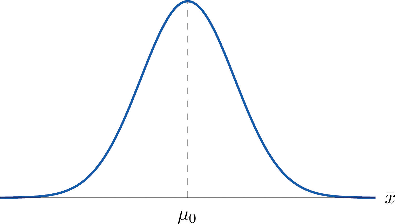
Supposing for now that $\bar{X}$ follows a normal distribution, when the null hypothesis is true the density function for the sample mean $\bar{X}$ must be as in Figure 8.1 "The Density Curve for ": a bell curve centered at $μ_0$ . Thus if $H_0$ is true then $\bar{X}$ - is likely to take a value near $μ_0$ and is unlikely to take values far away. Our decision procedure therefore reduces simply to:

if $H_a$ has the form $H_a:μ<μ_0$ then reject $H_0$ if $\bar{x}$ is far to the left of $μ_0$ ;
if $H_a$ has the form $H_a:μ>μ_0$ then reject $H_0$ if $\bar{x}$ is far to the right of $μ_0$ ;
if $H_a$ has the form $H_a:μ \neμ_0$ then reject $H_0$ if $\bar{x}$ is far away from $μ_0$ in either direction.

Figure 8.1 The Density Curve for $\bar{X}$ if $H_0$ Is True

Think of the respirator example, for which the null hypothesis is $H_0:μ=75$ , the claim that the average time air is delivered for all respirators is 75 minutes. If the sample mean is 75 or greater then we certainly would not reject $H_0$ (since there is no issue with an emergency respirator delivering air even longer than claimed).

If the sample mean is slightly less than 75 then we would logically attribute the difference to sampling error and also not reject $H_0$ either.

Values of the sample mean that are smaller and smaller are less and less likely to come from a population for which the population mean is 75. Thus if the sample mean is far less than 75, say around 60 minutes or less, then we would certainly reject $H_0$ , because we know that it is highly unlikely that the average of a sample would be so low if the population mean were 75. This is the rare event criterion for rejection: what we actually observed ( $\bar{X}<60$ ) would be so rare an event if $μ = 75$ were true that we regard it as much more likely that the alternative hypothesis $μ <75$ holds.

In summary, to decide between $H_0$ and $H_a$ in this example we would select a “rejection region” of values sufficiently far to the left of 75, based on the rare event criterion, and reject $H_0$ if the sample mean $\bar{X}$ lies in the rejection region, but not reject $H_0$ if it does not.

3. The Rejection Region

Each different form of the alternative hypothesis $H_a$ has its own kind of rejection region:

if (as in the respirator example) $H_a$ has the form $H_a:μ<μ_0$ , we reject $H_0$ if $\bar{X}$ is far to the left of $μ_0$ , that is, to the left of some number $C$ , so the rejection region has the form of an interval $(−∞,C]$ ;
if (as in the textbook example) $H_a$ has the form $H_a:μ>μ_0$ , we reject $H_0$ if $\bar{X}$ is far to the right of $μ_0$ , that is, to the right of some number $C$ , so the rejection region has the form of an interval $[C,∞)$ ;
if (as in the baked good example) $H_a$ has the form $H_a:μ \neμ_0$ , we reject $H_0$ if $\bar{X}$ is far away from $μ_0$ in either direction, that is, either to the left of some number $C$ or to the right of some other number $C'$ , so the rejection region has the form of the union of two intervals $(−∞,C]∪[C′,∞)$ .

The key issue in our line of reasoning is the question of how to determine the number $C$ or numbers $C$ and $C'$ , called the critical value or critical values of the statistic, that determine the rejection region.

The critical value or critical values of a test of hypotheses are the number or numbers that determine the rejection region.

Suppose the rejection region is a single interval, so we need to select a single number $C$ . Here is the procedure for doing so. We select a small probability, denoted $α$ , say 1%, which we take as our definition of “rare event:” an event is “rare” if its probability of occurrence is less than $α$ . (In all the examples and problems in this text the value of $α$ will be given already.)

The probability that $\bar{X}$ takes a value in an interval is the area under its density curve and above that interval, so as shown in Figure 8.2 (drawn under the assumption that H0 is true, so that the curve centers at $μ_0$ ) the critical value $C$ is the value of $\bar{X}$ that cuts off a tail area $α$ in the probability density curve of $\bar{X}$ .

When the rejection region is in two pieces, that is, composed of two intervals, the total area above both of them must be $α$ , so the area above each one is $α/2$ , as also shown in Figure 8.2.

Figure 8.2

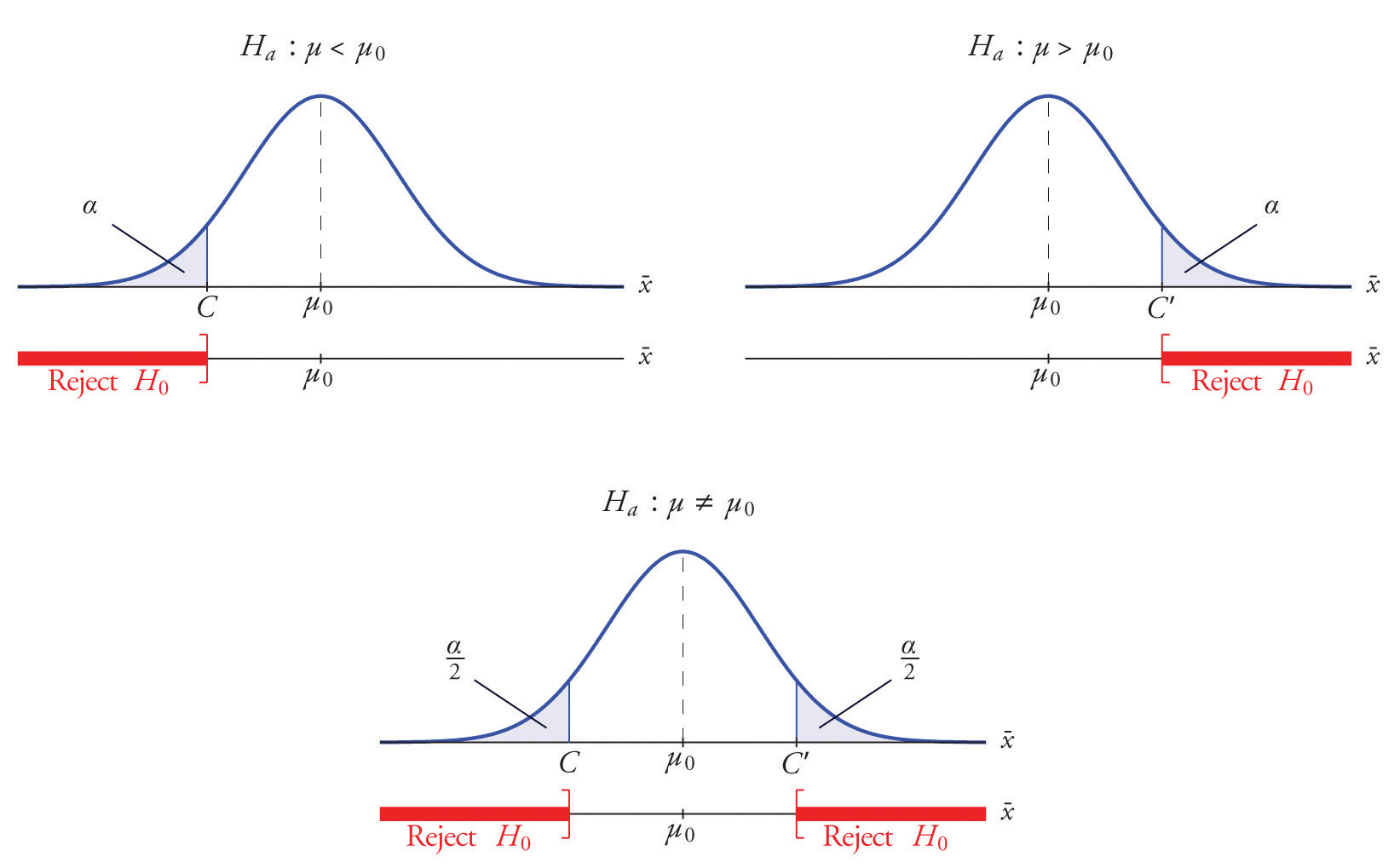
The number $α$ is the total area of a tail or a pair of tails.

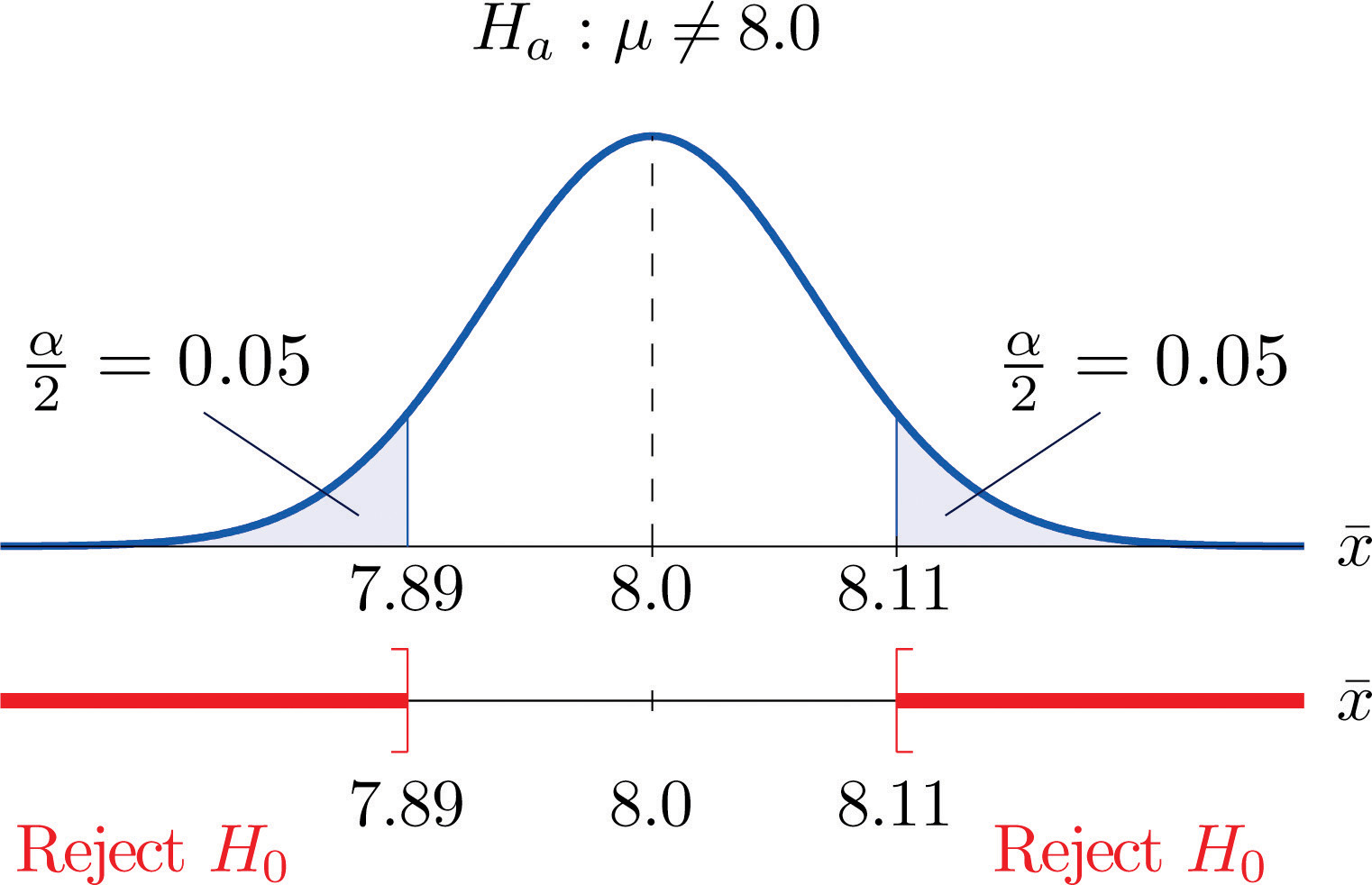
EXAMPLE 3. In the context of "EXAMPLE 2", suppose that it is known that the population is normally distributed with standard deviation $σ = 0.15$ gram, and suppose that the test of hypotheses $H_0:μ=8.0$ versus $H_a:μ≠8.0$ will be performed with a sample of size 5. Construct the rejection region for the test for the choice $α=0.10$ . Explain the decision procedure and interpret it.

[ Solution ]

,
$α=0.10$ , $(α∕2)=(0.10∕2)=0.05$ , $z_{0.05}=1.645$
so C and C′ are 1.645 standard deviations of $\bar{X}$ to the right and left of its mean 8.0

n <- 5
mu <- 8
sd <- 0.15
alpha <- 0.10

se <- sd / sqrt(n)

# in case of two-tail test
z <- qnorm(1-alpha/2); z

lc <- mu - z * se
uc <- mu + z * se

lc   # lower critical value
uc   # upper critical value

> z <- qnorm(1-alpha/2); z
## [1] 1.644854
> 
> lc <- mu - z * se
> uc <- mu + z * se
> 
> lc   # lower critical value
## [1] 7.88966
> uc   # upper critical value
## [1] 8.11034

Because the rejection regions are computed based on areas in tails of distributions, as shown in Figure 8.2, hypothesis tests are classified according to the form of the alternative hypothesis in the following way.

If $H_a$ has the form $H_a:μ \neμ_0$ the test is called a two-tailed test.
If $H_a$ has the form $H_a:μ < μ_0$ the test is called a left-tailed test.
If $H_a$ has the form $H_a:μ > μ_0$ the test is called a right-tailed test.
Each of the last two forms is also called a one-tailed test.

4. Two Types of Errors

The format of the testing procedure in general terms is to take a sample and use the information it contains to come to a decision about the two hypotheses. As stated before our decision will always be either

reject the null hypothesis $H_o$ in favor of the alternative $H_a$ presented, or
do not reject the null hypothesis $H_0$ in favor of the alternative $H_a$ presented.

There are four possible outcomes of hypothesis testing procedure, as shown in the following table:

True State of Nature

$Ho$ ia true

$Ho$ is false

Our Decision

Do not reject $Ho$

Correct decision

Type II error ( $\beta$ )

Reject $Ho$

Type I error ( $\alpha$ )

Correct Decision

As the table shows, there are two ways to be right and two ways to be wrong. Typically to reject $H_0$ when it is actually true is a more serious error than to fail to reject it when it is false, so the former error is labeled “Type I” and the latter error “Type II.”

In a test of hypotheses, a Type I error is the decision to reject $H_0$ when it is in fact true. A Type II error is the decision not to reject $H_0$ when it is in fact not true.

Unless we perform a census we do not have certain knowledge, so we do not know whether our decision matches the true state of nature or if we have made an error. We reject $H_0$ if what we observe would be a “rare” event if $H_0$ were true. But rare events are not impossible: they occur with probability $α$ . Thus when $H_0$ is true, a rare event will be observed in the proportion $α$ of repeated similar tests, and $H_0$ will be erroneously rejected in those tests. Thus $α$ is the probability that in following the testing procedure to decide between $H_0$ and $H_a$ we will make a Type I error.

The number $α$ that is used to determine the rejection region is called the level of significance of the test. It is the probability that the test procedure will result in a Type I error.

The probability of making a Type II error is too complicated to discuss in a beginning text, so we will say no more about it than this: for a fixed sample size, choosing $α$ smaller in order to reduce the chance of making a Type I error has the effect of increasing the chance of making a Type II error.

The only way to simultaneously reduce the chances of making either kind of error is to increase the sample size.

5. Standardizing the Test Statistic

Hypotheses testing will be considered in a number of contexts, and great unification as well as simplification results when the relevant sample statistic is standardized by subtracting its mean from it and then dividing by its standard deviation. The resulting statistic is called a standardized test statistic. In every situation treated in this and the following two chapters the standardized test statistic will have either the standard normal distribution or Student’s t-distribution.

A standardized test statistic for a hypothesis test is the statistic that is formed by subtracting from the statistic of interest its mean and dividing by its standard deviation.

For example, reviewing Note 8.14 "Example 3", if instead of working with the sample mean $\bar{X}$ we instead work with the test statistic $\frac{\bar{X}−8.0} {0.067} .$

then the distribution involved is standard normal and the critical values are just $±z_{0.05}$ . The extra work that was done to find that $C = 7.89$ and $C′=8.11$ is eliminated.

In every hypothesis test in this book the standardized test statistic will be governed by either the standard normal distribution or Student’s t-distribution. Information about rejection regions is summarized in the following tables:

When the test statistic has the standard normal distribution:

Symbol in Ha

Terminology

Rejection Region

$<$

Left-tailed test

$(−∞,−z_α]$

$>$

Right-tailed test

$[z_α,∞)$

$≠$

Two-tailed test

$(−∞,−z_{α∕2}]∪[z_{α∕2},∞)$

When the test statistic has Student’s t-distribution:

Symbol in Ha

Terminology

Rejection Region

$<$

Left-tailed test

$(−∞,−t_α]$

$>$

Right-tailed test

$[t_α,∞)$

$≠$

Two-tailed test

$(−∞,−t_{α∕2}]∪[t_{α∕2},∞)$

Every instance of hypothesis testing discussed in this and the following two chapters will have a rejection region like one of the six forms tabulated in the tables above.

No matter what the context a test of hypotheses can always be performed by applying the following systematic procedure, which will be illustrated in the examples in the succeeding sections.

Systematic Hypothesis Testing Procedure: Critical Value Approach
Identify the null and alternative hypotheses.
Identify the relevant test statistic and its distribution.
Compute from the data the value of the test statistic.
Construct the rejection region.
Compare the value computed in Step 3 to the rejection region constructed in Step 4 and make a decision. Formulate the decision in the context of the problem, if applicable.

The procedure that we have outlined in this section is called the “Critical Value Approach” to hypothesis testing to distinguish it from an alternative but equivalent approach that will be introduced at the end of Section 8.3 "The Observed Significance of a Test".

PreviousChapter 8. Testing Hypotheses Next8-1. Exercises

Last updated 4 years ago