11-3. F-tests for Equality of Two Variances

1. F-Distributions

Another important and useful family of distributions in statistics is the family of F-distributions. Each member of the F-distribution family is specified by a pair of parameters called degrees of freedom and denoted $df_1$ and $df_2$ . Figure 11.7 "Many " shows several F-distributions for different pairs of degrees of freedom. An F random variable is a random variable that assumes only positive values and follows an F-distribution.

Figure 11.7 Many F-Distributions

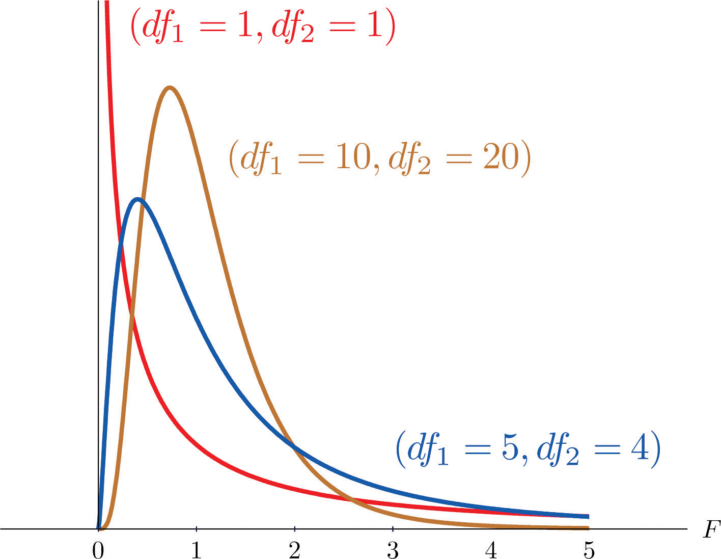
The parameter $df_1$ is often referred to as the numerator degrees of freedom and the parameter $df_2$ as the denominator degrees of freedom. It is important to keep in mind that they are not interchangeable. For example, the F-distribution with degrees of freedom $df_1=3$ and $df_2=8$ is a different distribution from the F-distribution with degrees of freedom $df_1=8$ and $df_2=3$.

The value of the F random variable F with degrees of freedom $df_1$ and $df_2$ that cuts off a right tail of area c is denoted $F_c$ and is called a critical value. See Figure 11.8.

Figure 11.8 $F_c$ Illustrated

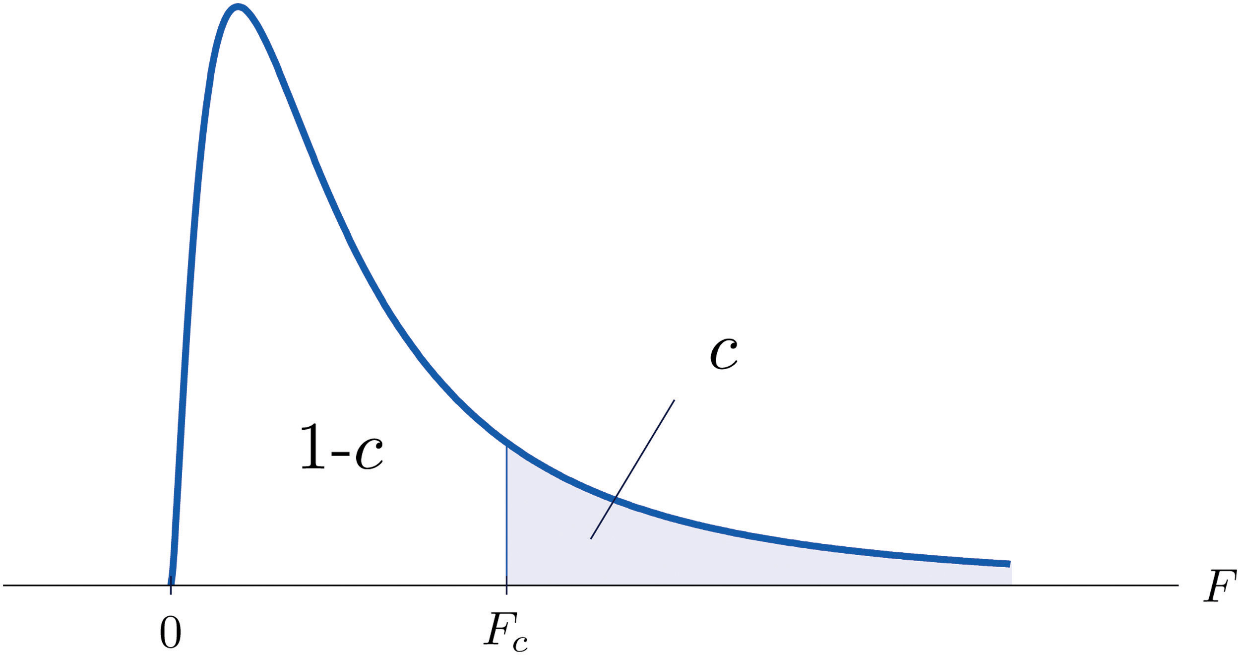
Tables containing the values of $F_c$ are given in Chapter 11 "Chi-Square Tests and ". Each of the tables is for a fixed collection of values of c, either 0.900, 0.950, 0.975, 0.990, and 0.995 (yielding what are called “lower” critical values), or 0.005, 0.010, 0.025, 0.050, and 0.100 (yielding what are called “upper” critical values). In each table critical values are given for various pairs $(df_1,df_2)$ . We illustrate the use of the tables with several examples.

F-Distribution Tables

EXAMPLE 3. Suppose F is an F random variable with degrees of freedom $df_1=5$ and $df_2=4$ . Use the tables to find

1. $F_{0.10}$

2. $F_{0.95}$

[ Solution ]

1. The column headings of all the tables contain $df_1=5$ . Look for the table for which 0.10 is one of the entries on the extreme left (a table of upper critical values) and that has a row heading $df_2=4$ in the left margin of the table. A portion of the relevant table is provided. The entry in the intersection of the column with heading $df_1=5$ and the row with the headings 0.10 and $df_2=4$, which is shaded in the table provided, is the answer, $F_{0.10}=4.05$ .

   F Tail Area	$df_1$	1	2	⋅ ⋅ ⋅  · · ·	5	⋅ ⋅ ⋅  · · ·
   $df_2$
   ⋮	⋮	⋮	⋮	⋮	⋮	⋮
   0.005	4	⋅ ⋅ ⋅  · · ·	⋅ ⋅ ⋅  · · ·	⋅ ⋅ ⋅  · · ·	22.5	⋅ ⋅ ⋅  · · ·
   0.01	4	⋅ ⋅ ⋅  · · ·	⋅ ⋅ ⋅  · · ·	⋅ ⋅ ⋅  · · ·	15.5	⋅ ⋅ ⋅  · · ·
   0.025	4	⋅ ⋅ ⋅  · · ·	⋅ ⋅ ⋅  · · ·	⋅ ⋅ ⋅  · · ·	9.36	⋅ ⋅ ⋅  · · ·
   0.05	4	⋅ ⋅ ⋅  · · ·	⋅ ⋅ ⋅  · · ·	⋅ ⋅ ⋅  · · ·	6.26	⋅ ⋅ ⋅  · · ·
   0.10	4	⋅ ⋅ ⋅  · · ·	⋅ ⋅ ⋅  · · ·	⋅ ⋅ ⋅  · · ·	$4.05$	⋅ ⋅ ⋅  · · ·
   ⋮	⋮	⋮	⋮	⋮	⋮	⋮

2. Look for the table for which 0.95 is one of the entries on the extreme left (a table of lower critical values) and that has a row heading $df_2=4$ in the left margin of the table. A portion of the relevant table is provided. The entry in the intersection of the column with heading $df_1=5$ and the row with the headings 0.95 and $df_2=4$, which is shaded in the table provided, is the answer, $F_{0.95}=0.19$ .

   F Tail Area	$df_1$	1	2	⋅ ⋅ ⋅  · · ·	5	⋅ ⋅ ⋅  · · ·
   $df_2$
   ⋮	⋮	⋮	⋮	⋮	⋮	⋮
   0.90	4	⋅ ⋅ ⋅  · · ·	⋅ ⋅ ⋅  · · ·	⋅ ⋅ ⋅  · · ·	0.28	⋅ ⋅ ⋅  · · ·
   0.95	4	⋅ ⋅ ⋅  · · ·	⋅ ⋅ ⋅  · · ·	⋅ ⋅ ⋅  · · ·	$0.19$	⋅ ⋅ ⋅  · · ·
   0.975	4	⋅ ⋅ ⋅  · · ·	⋅ ⋅ ⋅  · · ·	⋅ ⋅ ⋅  · · ·	0.14	⋅ ⋅ ⋅  · · ·
   0.99	4	⋅ ⋅ ⋅  · · ·	⋅ ⋅ ⋅  · · ·	⋅ ⋅ ⋅  · · ·	0.09	⋅ ⋅ ⋅  · · ·
   0.995	4	⋅ ⋅ ⋅  · · ·	⋅ ⋅ ⋅  · · ·	⋅ ⋅ ⋅  · · ·	0.06	⋅ ⋅ ⋅  · · ·
   ⋮	⋮	⋮	⋮	⋮	⋮	⋮

R Source

library(Rstat)

df_1 <- 5
df_2 <- 4

pv <- c(0.90, 0.05)
f.quant(df_1, df_2, pv)

Result

EXAMPLE 4. Suppose $F$ is an F random variable with degrees of freedom $df_1=2$ and $df_2=20$. Let $α=0.05$ . Use the tables to find

1. $F_α$

2. $F_{α∕2}$

3. $F_{1−α}$

4. $F_{1−α∕2}$

[ Solution ]

1. The column headings of all the tables contain $df_1=2$ . Look for the table for which $α=0.05$ is one of the entries on the extreme left (a table of upper critical values) and that has a row heading $df_2=20$ in the left margin of the table. A portion of the relevant table is provided. The shaded entry, in the intersection of the column with heading $df_1=2$ and the row with the headings 0.05 and $df_2=20$ is the answer, $F_{0.05}=3.49$ .

   F Tail Area	$df_1$	1	2	⋅ ⋅ ⋅  · · ·
   $df_2$
   ⋮	⋮	⋮	⋮	⋮
   0.005	20	⋅ ⋅ ⋅  · · ·	6.99	⋅ ⋅ ⋅  · · ·
   0.01	20	⋅ ⋅ ⋅  · · ·	5.85	⋅ ⋅ ⋅  · · ·
   0.025	20	⋅ ⋅ ⋅  · · ·	4.46	⋅ ⋅ ⋅  · · ·
   0.05	20	⋅ ⋅ ⋅  · · ·	$3.49$	⋅ ⋅ ⋅  · · ·
   0.10	20	⋅ ⋅ ⋅  · · ·	2.59	⋅ ⋅ ⋅  · · ·
   ⋮	⋮	⋮	⋮	⋮

2. Look for the table for which $α∕2=0.025$ is one of the entries on the extreme left (a table of upper critical values) and that has a row heading $df_2=20$ in the left margin of the table. A portion of the relevant table is provided. The shaded entry, in the intersection of the column with heading $df_1=2$ and the row with the headings 0.025 and $df_2=20$ is the answer, $F_{0.025}=4.46$ .

   F Tail Area	$df_1$	1	2	⋅ ⋅ ⋅  · · ·
   $df_2$
   ⋮	⋮	⋮	⋮	⋮
   0.005	20	⋅ ⋅ ⋅  · · ·	6.99	⋅ ⋅ ⋅  · · ·
   0.01	20	⋅ ⋅ ⋅  · · ·	5.85	⋅ ⋅ ⋅  · · ·
   0.025	20	⋅ ⋅ ⋅  · · ·	$4.46$	⋅ ⋅ ⋅  · · ·
   0.05	20	⋅ ⋅ ⋅  · · ·	3.49	⋅ ⋅ ⋅  · · ·
   0.10	20	⋅ ⋅ ⋅  · · ·	2.59	⋅ ⋅ ⋅  · · ·
   ⋮	⋮	⋮	⋮	⋮

3. Look for the table for which $(1−α)=0.95$ is one of the entries on the extreme left (a table of lower critical values) and that has a row heading $df_2=20$ in the left margin of the table. A portion of the relevant table is provided. The shaded entry, in the intersection of the column with heading $df_1=2$ and the row with the headings 0.95 and $df_2=20$ is the answer, F0.95=0.05.F0.95=0.05.

   F Tail Area	$df_1$	1	2	⋅ ⋅ ⋅  · · ·
   $df_2$
   ⋮	⋮	⋮	⋮	⋮
   0.90	20	⋅ ⋅ ⋅  · · ·	0.11	⋅ ⋅ ⋅  · · ·
   0.95	20	⋅ ⋅ ⋅  · · ·	$0.05$	⋅ ⋅ ⋅  · · ·
   0.975	20	⋅ ⋅ ⋅  · · ·	0.03	⋅ ⋅ ⋅  · · ·
   0.99	20	⋅ ⋅ ⋅  · · ·	0.01	⋅ ⋅ ⋅  · · ·
   0.995	20	⋅ ⋅ ⋅  · · ·	0.01	⋅ ⋅ ⋅  · · ·
   ⋮	⋮	⋮	⋮	⋮

4. Look for the table for which $(1−α∕2)=0.975$ is one of the entries on the extreme left (a table of lower critical values) and that has a row heading $df_2=20$ in the left margin of the table. A portion of the relevant table is provided. The shaded entry, in the intersection of the column with heading $df_1=2$ and the row with the headings 0.975 and $df_2=20$ is the answer, $F_{0.975}=0.03$ .

   F Tail Area	$df_1$	1	2	⋅ ⋅ ⋅  · · ·
   $df_2$
   ⋮	⋮	⋮	⋮	⋮
   0.90	20	⋅ ⋅ ⋅  · · ·	0.11	⋅ ⋅ ⋅  · · ·
   0.95	20	⋅ ⋅ ⋅  · · ·	0.05	⋅ ⋅ ⋅  · · ·
   0.975	20	⋅ ⋅ ⋅  · · ·	$0.03$	⋅ ⋅ ⋅  · · ·
   0.99	20	⋅ ⋅ ⋅  · · ·	0.01	⋅ ⋅ ⋅  · · ·
   0.995	20	⋅ ⋅ ⋅  · · ·	0.01	⋅ ⋅ ⋅  · · ·
   ⋮	⋮	⋮	⋮	⋮

R Source

library(Rstat)

df_1 <- 2
df_2 <- 20

pv <- c(0.95, 0.975, 0.05, 0.025)
f.quant(df_1, df_2, pv)

Result

A fact that sometimes allows us to find a critical value from a table that we could not read otherwise is:

If $F_u(r,s)$ denotes the value of the F-distribution with degrees of freedom $df_1=r$ and $df_2=s$

that cuts off a right tail of area u, then

$F_c(k,ℓ)= \frac {1}{F_{1−c}(ℓ,k)}$

EXAMPLE 5. Use the tables to find

1. $F_{0.01}$ for an F random variable with $df_1=13$ and $df_2=8$

2. $F_{0.975}$ for an F random variable with $df_1=40$ and $df_2=10$

[ Solution ]

1. There is no table with $df_1=13$, but there is one with $df_2=8$. Thus we use the fact that $F_{0.01}(13, 8)= \frac{1}{F_{0.99}(8,13)}$

Using the relevant table we find that $F_{0.99}(8,13)=0.18$ , hence $F_{0.01}(13,8)=0.18^{-1} = 5.556.$

R Source

library(Rstat)

df_1 <- 13
df_2 <- 8
alpha <- 0.01

pv <- c(1-alpha)
f.quant(df_1, df_2, pv)

pv_1 <- c(alpha)
f.quant(df_2, df_1, pv_1)

Result

2. There is no table with $df_1=40$, but there is one with $df_2=10$. Thus we use the fact that $F_{0.975}(40,10)= \frac{1}{F_{0.025}(10,40)}$

Using the relevant table we find that $F_{0.025}(10,40)=2.3882$ , hence $F_{0.975}(10,40)=2.3882^{-1}=0.4187$

R Source

library(Rstat)

df_1 <- 40
df_2 <- 10
alpha <- 0.975

pv <- c(1-alpha)
f.quant(df_1, df_2, pv)

pv_1 <- c(alpha)
f.quant(df_2, df_1, pv_1)

Result

2. F-Tests for Equality of Two Variances

In Chapter 9 "Two-Sample Problems" we saw how to test hypotheses about the difference between two population means $μ_1$ and $μ_2$ . In some practical situations the difference between the population standard deviations $σ_1$ and $σ_2$ is also of interest. Standard deviation measures the variability of a random variable. For example, if the random variable measures the size of a machined part in a manufacturing process, the size of standard deviation is one indicator of product quality. A smaller standard deviation among items produced in the manufacturing process is desirable since it indicates consistency in product quality.

For theoretical reasons it is easier to compare the squares of the population standard deviations, the population variances $σ_1^2$ and $σ_2^2$. This is not a problem, since $σ_1=σ_2$ precisely when $σ^2_1=σ_2^2$ , $σ_1<σ_2$ precisely when $σ_1^2<σ_2^2$ , and $σ_1>σ_2$ precisely when $σ_1^2>σ_2^2$ .

The null hypothesis always has the form $H_0:σ_1=σ_2$. The three forms of the alternative hypothesis, with the terminology for each case, are:

Form of $H_a$	Terminology
$H_a:σ_1^2>σ_2^2$	Right-tailed
$H_a:σ_1^2<σ_2^2$	Left-tailed
$H_a:σ_1^2 \ne σ_2^2$	Two-tailed

Just as when we test hypotheses concerning two population means, we take a random sample from each population, of sizes $n_1$ and $n_2$ , and compute the sample standard deviations $s_1$ and $s_2$ . In this context the samples are always independent. The populations themselves must be normally distributed.

Test Statistic for Hypothesis Tests Concerning the Difference Between Two Population Variances

$F= \frac{s^2_1}{s_2^2}$

If the two populations are normally distributed and if $H_0:σ^2_1=σ_2^2$ is true then under independent sampling F approximately follows an F-distribution with degrees of freedom $df_1=(n_1−1)$ and $df_2=(n_2−1)$ .

A test based on the test statistic $F$ is called an F-test.

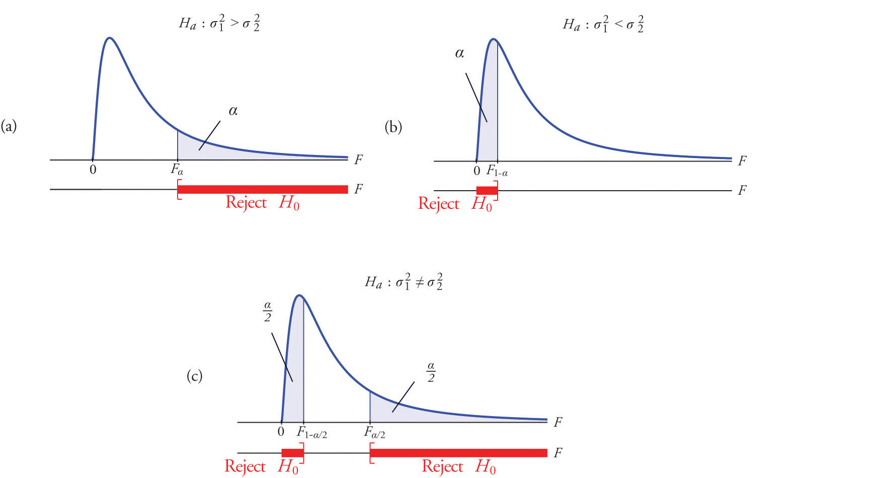
A most important point is that while the rejection region for a right-tailed test is exactly as in every other situation that we have encountered, because of the asymmetry in the F-distribution the critical value for a left-tailed test and the lower critical value for a two-tailed test have the special forms shown in the following table:

Terminology	Alternative Hypothesis	Rejection Region
Right-tailed	$H_a:σ_1^2>σ_2^2$	$F≥F_α$
Left-tailed	$H_a:σ_1^2<σ_2^2$	$F≤F_{1−α}$
Two-tailed	$H_a:σ_1^2 \ne σ_2^2$	$F≤F_{1−α∕2} \space or \space F≥F_{α∕2}$

Figure 11.9 "Rejection Regions: (a) Right-Tailed; (b) Left-Tailed; (c) Two-Tailed" illustrates these rejection regions.

Figure 11.9 Rejection Regions: (a) Right-Tailed; (b) Left-Tailed; (c) Two-Tailed

The test is performed using the usual five-step procedure described at the end of Section 8.1 "The Elements of Hypothesis Testing" in Chapter 8 "Testing Hypotheses".

EXAMPLE 6. One of the quality measures of blood glucose meter strips is the consistency of the test results on the same sample of blood. The consistency is measured by the variance of the readings in repeated testing. Suppose two types of strips, A and B, are compared for their respective consistencies. We arbitrarily label the population of Type A strips Population 1 and the population of Type B strips Population 2. Suppose 15 Type A strips were tested with blood drops from a well-shaken vial and 20 Type B strips were tested with the blood from the same vial. The results are summarized in Table 11.16 "Two Types of Test Strips". Assume the glucose readings using Type A strips follow a normal distribution with variance σ21σ12 and those using Type B strips follow a normal distribution with variance with σ22.σ22. Test, at the 10% level of significance, whether the data provide sufficient evidence to conclude that the consistencies of the two types of strips are different.

TABLE 11.16 TWO TYPES OF TEST STRIPS

Strip Type	Sample Size	Sample Variance
A	$n_1=16$	$s_1^2=2.09$
B	$n_2=21$	$s_2^2=1.10$

[ Solution ]

• Step 1. The test of hypotheses is $H_0:σ_1=σ_2$ vs. $H_a:σ_1^2 \ne σ_2^2 \space \space @ α=0.10$

• Step 2. The distribution is the F-distribution with degrees of freedom

  $df_1=(16−1)=15$ and $df_2=(21−1)=20$ .

• Step 3. The test is two-tailed. The left or lower critical value is $F_{1−α∕2}=F_{0.95}=0.43$ . The right or upper critical value is $F_{α∕2}=F_{0.05}=2.20$ . Thus the rejection region is $[0,−0.43]∪[2.20,∞)$ , as illustrated in Figure 11.10 "Rejection Region and Test Statistic for ".

Figure 11.10 Rejection Region and Test Statistic for Note 11.27 "Example 6"

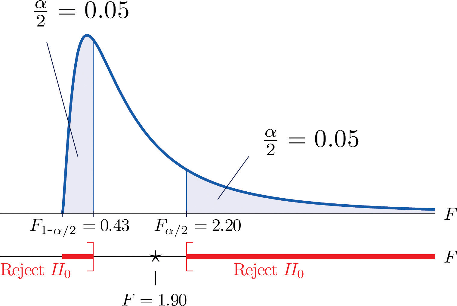
• Step 4. The value of the test statistic is $F=\frac{s^2_1}{s^2_2}=\frac{2.09}{1.10}=1.90$

• Step 5. As shown in Figure 11.10 "Rejection Region and Test Statistic for ", the test statistic 1.90 does not lie in the rejection region, so the decision is not to reject $H_0$ .

• The data do not provide sufficient evidence, at the 10% level of significance, to conclude that there is a difference in the consistency, as measured by the variance, of the two types of test strips.

EXAMPLE 7. In the context of Note 11.27 "Example 6", suppose Type A test strips are the current market leader and Type B test strips are a newly improved version of Type A. Test, at the 10% level of significance, whether the data given in Table 11.16 "Two Types of Test Strips" provide sufficient evidence to conclude that Type B test strips have better consistency (lower variance) than Type A test strips.

[ Solution ]

• Step 1. The test of hypotheses is now $H_0:σ_1=σ_2$ vs. $H_a:σ_1^2 \ne σ_2^2 \space \space @ α=0.10$

• Step 2. The distribution is the F-distribution with degrees of freedom

  $df_1=(16−1)=15$ and $df_2=(21−1)=20$

• Step 3. The value of the test statistic is $F=\frac{s^2_1}{s^2_2}=\frac{2.09}{1.10}=1.90$

• Step 4. The test is right-tailed. The single critical value is $F_α=F_{0.10}=1.84$

  Thus the rejection region is $[1.84,∞)$, as illustrated in Figure 11.11 "Rejection Region and Test Statistic for ".

Figure 11.11 Rejection Region and Test Statistic for Note 11.28 "Example 7"

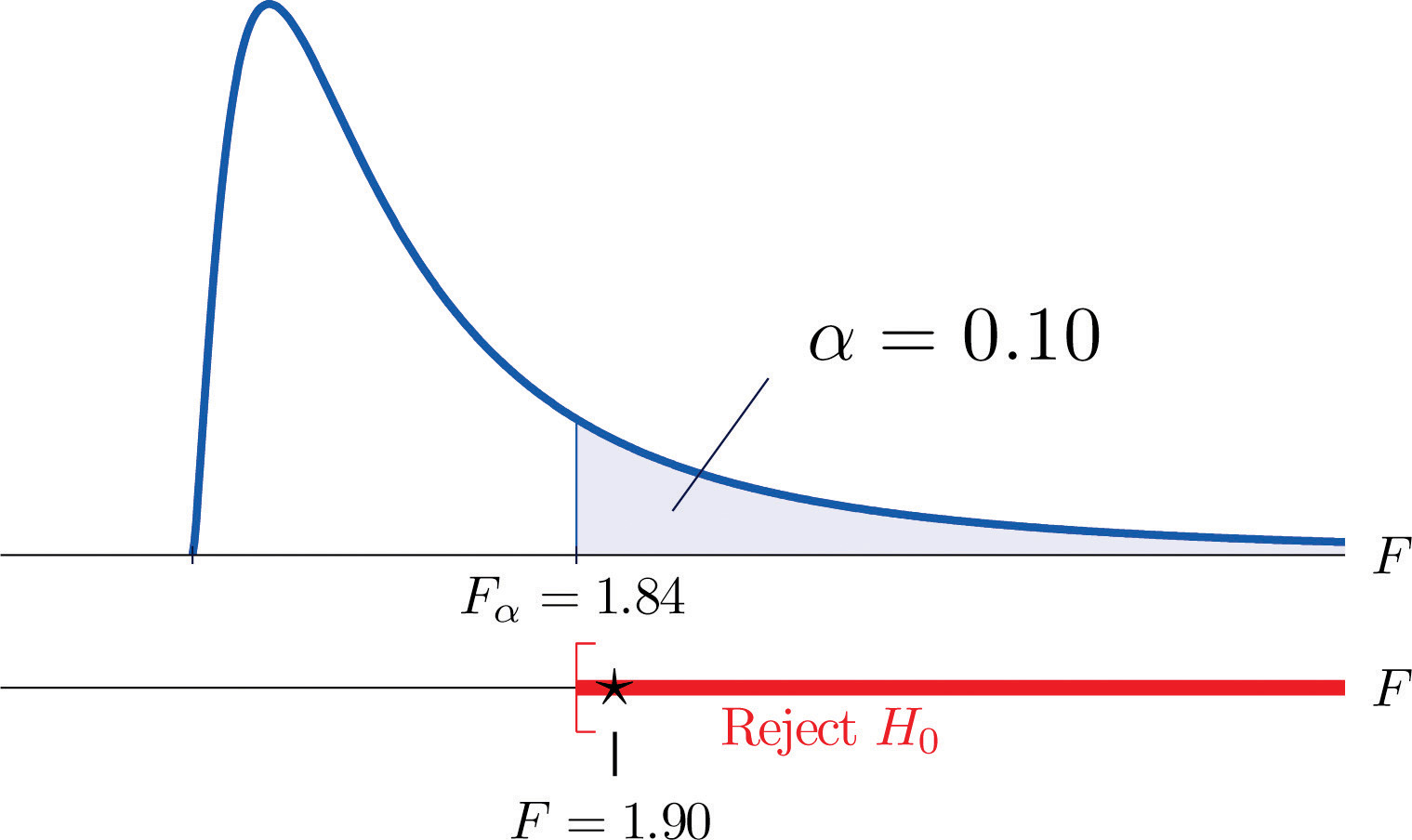
• Step 5. As shown in Figure 11.11 "Rejection Region and Test Statistic for ", the test statistic 1.90 lies in the rejection region, so the decision is to reject $H_0$ .

• The data provide sufficient evidence, at the 10% level of significance, to conclude that Type B test strips have better consistency (lower variance) than Type A test strips do.