9-3. Comparison of Two Population Means: Paired Samples

Suppose chemical engineers wish to compare the fuel economy obtained by two different formulations of gasoline. Since fuel economy varies widely from car to car, if the mean fuel economy of two independent samples of vehicles run on the two types of fuel were compared, even if one formulation were better than the other the large variability from vehicle to vehicle might make any difference arising from difference in fuel difficult to detect. Just imagine one random sample having many more large vehicles than the other. Instead of independent random samples, it would make more sense to select pairs of cars of the same make and model and driven under similar circumstances, and compare the fuel economy of the two cars in each pair. Thus the data would look something like Table 9.1 "Fuel Economy of Pairs of Vehicles", where the first car in each pair is operated on one formulation of the fuel (call it Type 1 gasoline) and the second car is operated on the second (call it Type 2 gasoline).

Table 9.1 Fuel Economy of Pairs of Vehicles

Make and Model	Car 1	Car 2
Buick LaCrosse	17.0	17.0
Dodge Viper	13.2	12.9
Honda CR-Z	35.3	35.4
Hummer H 3	13.6	13.2
Lexus RX	32.7	32.5
Mazda CX-9	18.4	18.1
Saab 9-3	22.5	22.5
Toyota Corolla	26.8	26.7
Volvo XC 90	15.1	15.0

The first column of numbers form a sample from Population 1, the population of all cars operated on Type 1 gasoline; the second column of numbers form a sample from Population 2, the population of all cars operated on Type 2 gasoline. It would be incorrect to analyze the data using the formulas from the previous section, however, since the samples were not drawn independently. What is correct is to compute the difference in the numbers in each pair (subtracting in the same order each time) to obtain the third column of numbers as shown in Table 9.2 "Fuel Economy of Pairs of Vehicles" and treat the differences as the data. At this point, the new sample of differences $d_1=0.0, \space …, \space d_9=0.1$ in the third column of Table 9.2 "Fuel Economy of Pairs of Vehicles" may be considered as a random sample of size $n = 9$ selected from a population with mean $μ_d=μ_1−μ_2.$ This approach essentially transforms the paired two-sample problem into a one-sample problem as discussed in the previous two chapters.

Table 9.2 Fuel Economy of Pairs of Vehicles

Make and Model	Car 1	Car 2	Difference
Buick LaCrosse	17.0	17.0	0.0
Dodge Viper	13.2	12.9	0.3
Honda CR-Z	35.3	35.4	−0.1
Hummer H 3	13.6	13.2	0.4
Lexus RX	32.7	32.5	0.2
Mazda CX-9	18.4	18.1	0.3
Saab 9-3	22.5	22.5	0.0
Toyota Corolla	26.8	26.7	0.1
Volvo XC 90	15.1	15.0	0.1

Note carefully that although it does not matter what order the subtraction is done, it must be done in the same order for all pairs. This is why there are both positive and negative quantities in the third column of numbers in Table 9.2 "Fuel Economy of Pairs of Vehicles".

1. Confidence Intervals

When the population of differences is normally distributed the following formula for a confidence interval for $μ_d=μ_1−μ_2$ is valid.

100(1−α)%100(1−α)% Confidence Interval for the Difference Between Two Population Means: Paired Difference Samples

$\bar{d} ± t_{α∕2} \frac{s_d} {\sqrt{n}}$

where there are n pairs, $\bar {d}$ is the mean and $s_d$ is the standard deviation of their differences.

The number of degrees of freedom is $df=n−1.$

The population of differences must be normally distributed.

EXAMPLE 7. Using the data in Table 9.1 "Fuel Economy of Pairs of Vehicles" construct a point estimate and a 95% confidence interval for the difference in average fuel economy between cars operated on Type 1 gasoline and cars operated on Type 2 gasoline.

[ Solution ]

The mean and standard deviation of the differences are

$\bar{d} = \frac {\Sigma}{n} = \frac{1.3}{9} =0.14$

and $s_d= \sqrt{\frac{(Σd^2−\frac{1}{n}(Σd)^2)} {n−1}} =\sqrt{ \frac{0.41− \frac{1}{9} (1.3)^2} {8} }=0.16$

The point estimate of $μ_1−μ_2 =μ_d$ is

$\bar{d} = 0.14$

In words, we estimate that the average fuel economy of cars using Type 1 gasoline is 0.14 mpg greater than the average fuel economy of cars using Type 2 gasoline.

To apply the formula for the confidence interval, we must find $t_{α∕2}.$ The 95% confidence level means that $α=(1−0.95)=0.05$ so that $t_{α∕2}=t_{0.025}.$ From Figure 12.3 "Critical Values of ", in the row with the heading $df=(9−1)=8$ we read that $t_{0.025}=2.306.$

Thus

$\bar{d} ± t_{α∕2} \frac{s_d} {\sqrt{n}} = 0.14±2.306( \frac {0.16} { \sqrt{9}} )≈0.14±0.13$

We are 95% confident that the difference in the population means lies in the interval $[0.01,0.27]$ , in the sense that in repeated sampling 95% of all intervals constructed from the sample data in this manner will contain $μ_d=μ_1−μ_2$. Stated differently, we are 95% confident that mean fuel economy is between 0.01 and 0.27 mpg greater with Type 1 gasoline than with Type 2 gasoline.

2. Hypothesis Testing

Testing hypotheses concerning the difference of two population means using paired difference samples is done precisely as it is done for independent samples, although now the null and alternative hypotheses are expressed in terms of μdμd instead of $(μ_1−μ_2).$ Thus the null hypothesis will always be written $H_0:μ_d=D_0.$

The three forms of the alternative hypothesis, with the terminology for each case, are:

Form of $H_a$	Terminology
$H_a:μ_d<D_0$	Left-tailed
$H_a:μ_d>D_0$	Right-tailed
$H_a:μ_d \ne D_0$	Two-tailed

The same conditions on the population of differences that was required for constructing a confidence interval for the difference of the means must also be met when hypotheses are tested. Here is the standardized test statistic that is used in the test.

Standardized Test Statistic for Hypothesis Tests Concerning the Difference Between Two Population Means: Paired Difference Samples

$t_o= \frac{ \bar{d} −D_0} {s_d/ \sqrt{n} }$

where there are $n$ pairs, $\bar{d}$ is the mean and $s_d$ is the standard deviation of their differences.

The test statistic has Student’s t-distribution with $df=(n−1)$ degrees of freedom.

The population of differences must be normally distributed.

EXAMPLE 8. Using the data of Table 9.2 "Fuel Economy of Pairs of Vehicles" test the hypothesis that mean fuel economy for Type 1 gasoline is greater than that for Type 2 gasoline against the null hypothesis that the two formulations of gasoline yield the same mean fuel economy. Test at the 5% level of significance using the critical value approach.

[ Solution ]

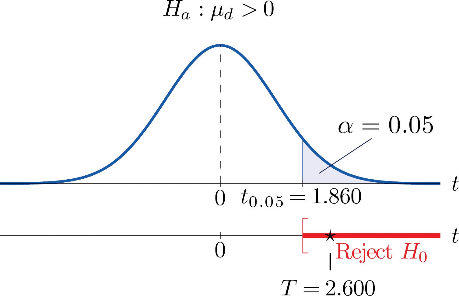
• Step 1. Since the differences were computed in the order  (Type 1 mpg− Type 2 mpg ) $μ_d=(μ_1−μ_2)>0.$ Thus the test is $H_0:μ_d=0 vs. \space H_a:μ_d>0, @ α=0.05$

  (If the differences had been computed in the opposite order then the alternative hypotheses would have been $H_a:μ_d<0.$ )

• Step 2. Since the sampling is in pairs the test statistic is $t_o= \frac{ \bar{d} −D_0} {s_d/ \sqrt{n} }$

• Step 3. We have already computed $\bar{d}$ and $s_d$ in the previous example. Inserting their values and $D_0=0$ into the formula for the test statistic gives $t_o= \frac{ \bar{d} −D_0} {s_d/ \sqrt{n} } = \frac{0.14} { 0.16/ 3}=2.600$

• Step 4. Since the symbol in $H_a$ is “ $>$ ” this is a right-tailed test, so there is a single critical value, $t_α=t_{0.05}$ with 8 degrees of freedom, which from the row labeled $df=8$ in Figure 12.3 "Critical Values of " we read off as 1.860. The rejection region is $[1.860,∞).$

• Step 5. As shown in Figure 9.5 "Rejection Region and Test Statistic for " the test statistic falls in the rejection region. The decision is to reject $H_0.$

• In the context of the problem our conclusion is:

  The data provide sufficient evidence, at the 5% level of significance, to conclude that the mean fuel economy provided by Type 1 gasoline is greater than that for Type 2 gasoline.

• Figure 9.5 Rejection Region and Test Statistic for Note 9.20 "Example 8"

EXAMPLE 9. Perform the test of Note 9.20 "Example 8" using the p-value approach.

[ Solution ]

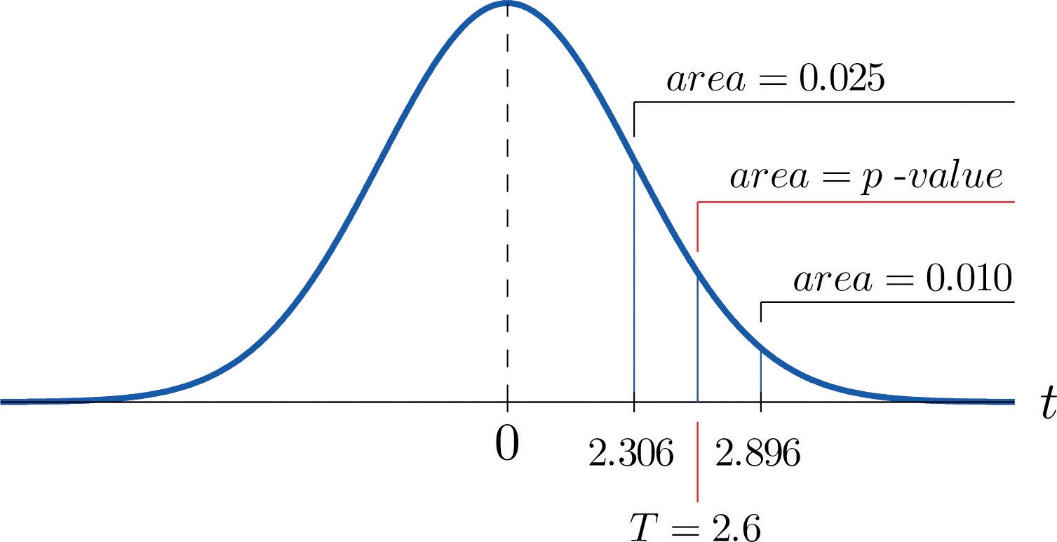
• Step 4. Because the test is one-tailed the observed significance or p-value of the test is just the area of the right tail of Student’s t-distribution, with 8 degrees of freedom, that is cut off by the test statistic $t_o = 2.600$ . We can only approximate this number. Looking in the row of Figure 12.3 "Critical Values of " headed $df=8,$ the number 2.600 is between the numbers 2.306 and 2.896, corresponding to $t_{0.025}$ and $t_{0.010}$ .

  The area cut off by $t_c = 2.306$ is 0.025 and the area cut off by $t_c = 2.896$ is 0.010. Since 2.600 is between 2.306 and 2.896 the area it cuts off is between 0.025 and 0.010. Thus the p-value is between 0.025 and 0.010. In particular it is less than 0.025. See Figure 9.6.

Figure 9.6 p-Value for Note 9.21 "Example 9"

• Step 5. Since 0.025 < 0.05, $p<α$ so the decision is to reject the null hypothesis:

  The data provide sufficient evidence, at the 5% level of significance, to conclude that the mean fuel economy provided by Type 1 gasoline is greater than that for Type 2 gasoline.

The paired two-sample experiment is a very powerful study design. It bypasses many unwanted sources of “statistical noise” that might otherwise influence the outcome of the experiment, and focuses on the possible difference that might arise from the one factor of interest.

If the sample is large (meaning that $n ≥ 30$ ) then in the formula for the confidence interval we may replace $t_{α∕2}$ by $z_{α∕2}.$ For hypothesis testing when the number of pairs is at least 30, we may use the same statistic as for small samples for hypothesis testing, except now it follows a standard normal distribution, so we use the last line of Figure 12.3 "Critical Values of " to compute critical values, and p-values can be computed exactly with Figure 12.2 "Cumulative Normal Probability", not merely estimated using Figure 12.3 "Critical Values of ".