9-1. Comparison of Two Population Means: Large, Independent Samples

1MB

chapter-09.pptx

Open

Chapter 9 (Korean)

The previous two chapters treated the questions of estimating and making inferences about a parameter of a single population.

In this chapter we consider a comparison of parameters that belong to two different populations. For example, we might wish to compare the average income of all adults in one region of the country with the average income of those in another region, or we might wish to compare the proportion of all men who are vegetarians with the proportion of all women who are vegetarians.

We will study construction of confidence intervals and tests of hypotheses in four situations, depending on the parameter of interest, the sizes of the samples drawn from each of the populations, and the method of sampling. We also examine sample size considerations.

9.1 Comparison of Two Population Means: Large, Independent Samples

LEARNING OBJECTIVES

1. To understand the logical framework for estimating the difference between the means of two distinct populations and performing tests of hypotheses concerning those means.

2. To learn how to construct a confidence interval for the difference in the means of two distinct populations using large, independent samples.

3. To learn how to perform a test of hypotheses concerning the difference between the means of two distinct populations using large, independent samples.

Suppose we wish to compare the means of two distinct populations. Figure 9.1 "Independent Sampling from Two Populations" illustrates the conceptual framework of our investigation in this and the next section. Each population has a mean and a standard deviation.

We arbitrarily label one population as Population 1 and the other as Population 2, and subscript the parameters with the numbers 1 and 2 to tell them apart. We draw a random sample from Population 1 and label the sample statistics it yields with the subscript 1.

Without reference to the first sample we draw a sample from Population 2 and label its sample statistics with the subscript 2.

Figure 9.1 Independent Sampling from Two Populations

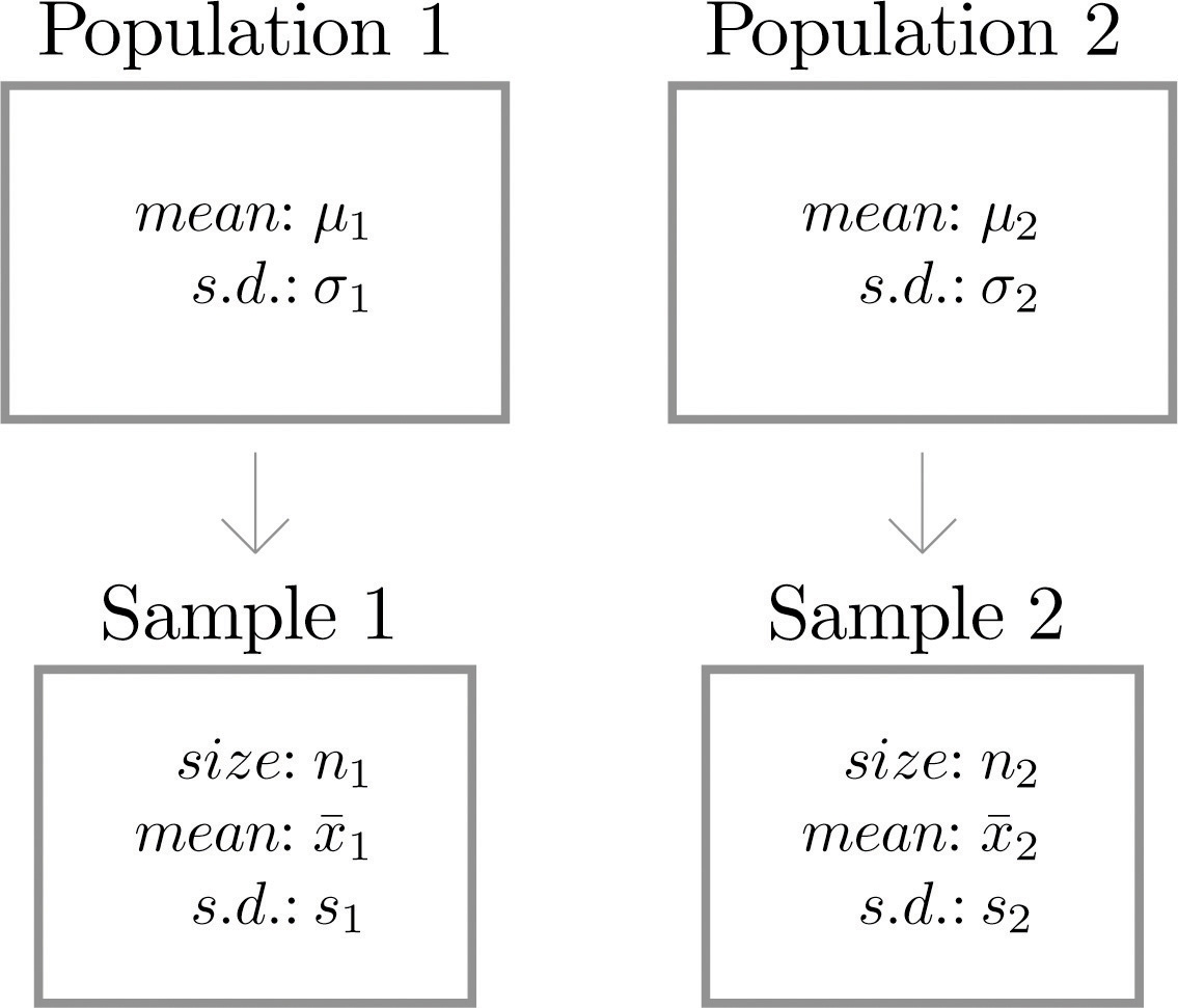
Samples from two distinct populations are independent if each one is drawn without reference to the other, and has no connection with the other.

Our goal is to use the information in the samples to estimate the difference $(μ1−μ2)$ in the means of the two populations and to make statistically valid inferences about it.

1. Confidence Intervals

Since the mean $\bar{x_1}$ of the sample drawn from Population 1 is a good estimator of $μ_1$ and the mean $\bar{x_2}$ of the sample drawn from Population 2 is a good estimator of $μ_2$, a reasonable point estimate of the difference $(μ_1- μ_2)$ is $(\bar{x_1}-\bar{x_2})$ .

In order to widen this point estimate into a confidence interval, we first suppose that both samples are large, that is, that both $n1≥30$ and $n2≥30.$ If so, then the following formula for a confidence interval for $(μ_1- μ_2)$ is valid.

The symbols $s_1^2$ and $s_2^2$ denote the squares of $s_1$ and $s_2$. (In the relatively rare case that both population standard deviations $σ1$ and $σ2$ are known they would be used instead of the sample standard deviations.)

100(1−α)%100(1−α)% Confidence Interval for the Difference Between Two Population Means: Large, Independent Samples

$(\bar{x_1}-\bar{x_2}) ±z_{\frac{α}{2}} \sqrt { \frac{s_1^2}{n_1} + \frac{s_2^2}{n_2} }$

The samples must be independent, and each sample must be large: $n_1≥30$ and $n_2≥30$ .

EXAMPLE 1. To compare customer satisfaction levels of two competing cable television companies, 174 customers of Company 1 and 355 customers of Company 2 were randomly selected and were asked to rate their cable companies on a five-point scale, with 1 being least satisfied and 5 most satisfied. The survey results are summarized in the following table:

Company 1	Company 2
$n_1=174$	$n_2=355$
$\bar{x_1}=3.51$	$\bar{x_2}=3.24$
$s_1=0.51$	$s_2=0.52$

Construct a point estimate and a 99% confidence interval for $(μ_1- μ_2)$, the difference in average satisfaction levels of customers of the two companies as measured on this five-point scale.

[ Solution ]

1. The point estimate of $(μ_1- μ_2)$ is $(\bar{x_1}-\bar{x_2}) =(3.51−3.24)=0.27.$ In words, we estimate that the average customer satisfaction level for Company 1 is 0.27 points higher on this five-point scale than it is for Company 2.

2. To apply the formula for the confidence interval, proceed exactly as was done in Chapter 7 "Estimation". The 99% confidence level means that $α=(1−0.99)=0.01$ so that $z_{α∕2}=z_{0.005}.$ From Figure 12.3 "Critical Values of " we read directly that $z_{0.005}=2.576.$ Thus $(\bar{x_1}-\bar{x_2}) ±z_{\frac{α}{2}} \sqrt { \frac{s_1^2}{n_1} + \frac{s_2^2}{n_2} }$ $= 0.27±2.576 \sqrt{\frac{0.51^2} {174}+ \frac{0.52^2}{355}}$ $= 0.27±0.12$

3. We are 99% confident that the difference in the population means lies in the interval $[0.15,0.39]$ , in the sense that in repeated sampling 99% of all intervals constructed from the sample data in this manner will contain $(μ_1- μ_2)$. In the context of the problem we say we are 99% confident that the average level of customer satisfaction for Company 1 is between 0.15 and 0.39 points higher, on this five-point scale, than that for Company 2.

2. Hypothesis Testing

Hypotheses concerning the relative sizes of the means of two populations are tested using the same critical value and p-value procedures that were used in the case of a single population. All that is needed is to know how to express the null and alternative hypotheses and to know the formula for the standardized test statistic and the distribution that it follows.

The null and alternative hypotheses will always be expressed in terms of the difference of the two population means. Thus the null hypothesis will always be written

$H_0:μ_1−μ_2=D_0$

where $D_0$ is a number that is deduced from the statement of the situation. As was the case with a single population the alternative hypothesis can take one of the three forms, with the same terminology:

Form of $H_a$	Terminology
$H_a:μ_1−μ_2<D_0$	Left-tailed
$H_a:μ_1−μ_2>D_0$	Right-tailed
$H_a:μ_1−μ_2 \ne D_0$	Two-tailed

As long as the samples are independent and both are large the following formula for the standardized test statistic is valid, and it has the standard normal distribution. (In the relatively rare case that both population standard deviations $σ_1$ and $σ_2$ are known they would be used instead of the sample standard deviations.)

Standardized Test Statistic for Hypothesis Tests Concerning the Difference Between Two Population Means: Large, Independent Samples

$z_o = \frac {(\bar{x_1}-\bar{x_2}) -D_0} { \sqrt { \frac{s_1^2}{n_1} + \frac{s_2^2}{n_2} }}$

The test statistic has the standard normal distribution.

The samples must be independent, and each sample must be large: $n1≥30$ and $n2≥30.$

EXAMPLE 2. Refer to Note 9.4 "Example 1" concerning the mean satisfaction levels of customers of two competing cable television companies. Test at the 1% level of significance whether the data provide sufficient evidence to conclude that Company 1 has a higher mean satisfaction rating than does Company 2. Use the critical value approach.

[ Solution ]

• Step 1. If the mean satisfaction levels $μ_1$ and $μ_2$ are the same then $μ_1 =μ_2$ , but we always express the null hypothesis in terms of the difference between $μ_1$ and $μ_2$ , hence $H_0$ is $μ_1−μ_2=0.$ To say that the mean customer satisfaction for Company 1 is higher than that for Company 2 means that $μ_1>μ_2$ , which in terms of their difference is $μ_1-μ_2>0$. The hypothsis test is therefore $H_0:μ_1−μ_2=0 \space vs. \space H_a:μ1−μ2>0, @ α=0.01$

• Step 2. Since the samples are independent and both are large the test statistic is $z_o = \frac {(\bar{x_1}-\bar{x_2}) -D_0} { \sqrt { \frac{s_1^2}{n_1} + \frac{s_2^2}{n_2} }}$

• Step 3. Inserting the data into the formula for the test statistic gives $z_o = \frac {(\bar{x_1}-\bar{x_2}) -D_0} { \sqrt { \frac{s_1^2}{n_1} + \frac{s_2^2}{n_2} }}$ $= \frac{(3.51−3.24)−0} { \frac{0.51^2} {174} + \frac {0.52^2}{355} } = 5.684$

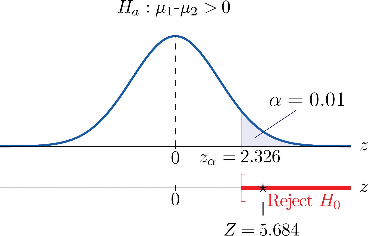
• Step 4. Since the symbol in $H_a$ is “ $>$ ” this is a right-tailed test, so there is a single critical value, $z_α=z_{0.01}$ , which from the last line in Figure 12.3 "Critical Values of " we read off as 2.326. The rejection region is $[2.326,∞).$ .

• Step 5. the test statistic falls in the rejection region. The decision is to reject $H_0$ .

• In the context of the problem our conclusion is: The data provide sufficient evidence, at the 1% level of significance, to conclude that the mean customer satisfaction for Company 1 is higher than that for Company 2.

Figure 9.2 Rejection Region and Test Statistic for Note 9.6 "Example 2"

EXAMPLE 3. Perform the test of Note 9.6 "Example 2" using the p-value approach.

[ Solution ]

The first three steps are identical to those in Note 9.6 "Example 2".

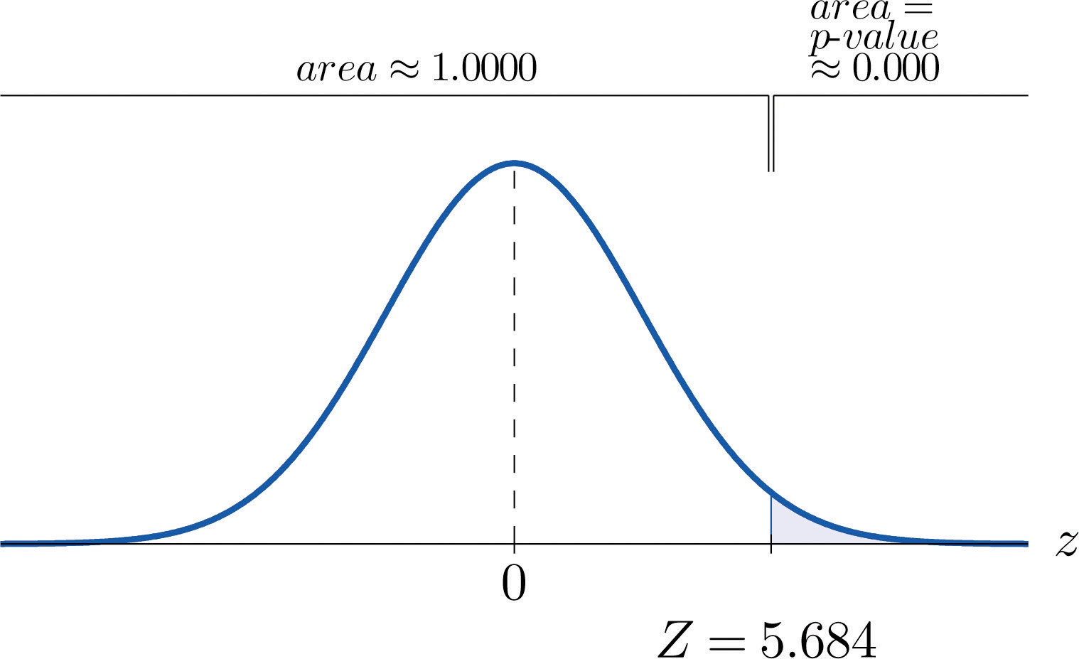
• Step 4. The observed significance or p-value of the test is the area of the right tail of the standard normal distribution that is cut off by the test statistic $z_o = 5.684.$ The number 5.684 is too large to appear in Figure 12.2 "Cumulative Normal Probability", which means that the area of the left tail that it cuts off is 1.0000 to four decimal places. The area that we seek, the area of the right tail, is therefore $(1−1.0000)=0.0000$ to four decimal places. See Figure 9.3. That is, $p -value=0.0000$ to four decimal places. (The actual value is approximately $0.000 000 007.$ )

Figure 9.3 P-Value for Note 9.7 "Example 3"

• Step 5. Since 0.0000 < 0.01, p -value $<α$ so the decision is to reject the null hypothesis:

  The data provide sufficient evidence, at the 1% level of significance, to conclude that the mean customer satisfaction for Company 1 is higher than that for Company 2.