10-6. The Coefficient of Determination

If the scatter diagram of a set of $(x,y)$ pairs shows neither an upward or downward trend, then the horizontal line $\hat{y}= \bar{y}$ fits it well, as illustrated in Figure 10.11.

The lack of any upward or downward trend means that when an element of the population is selected at random, knowing the value of the measurement $x$ for that element is not helpful in predicting the value of the measurement $y$ .

Figure 10.11

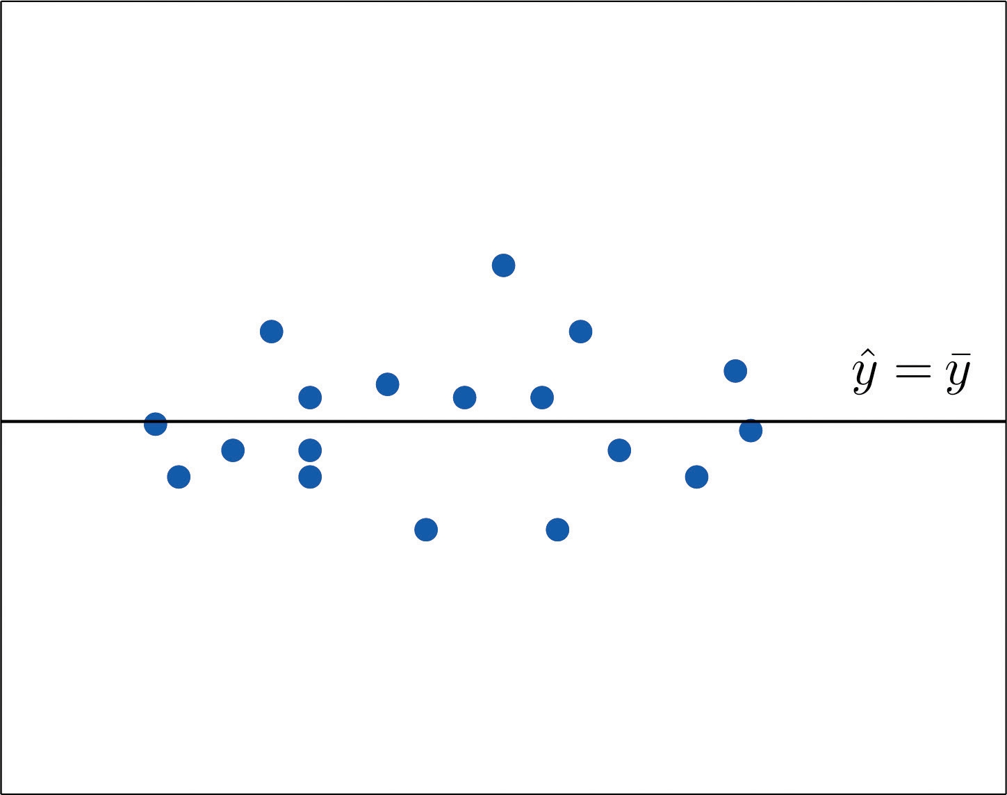
The line $\hat{y}= \bar{y}$ fits the scatter diagram well.

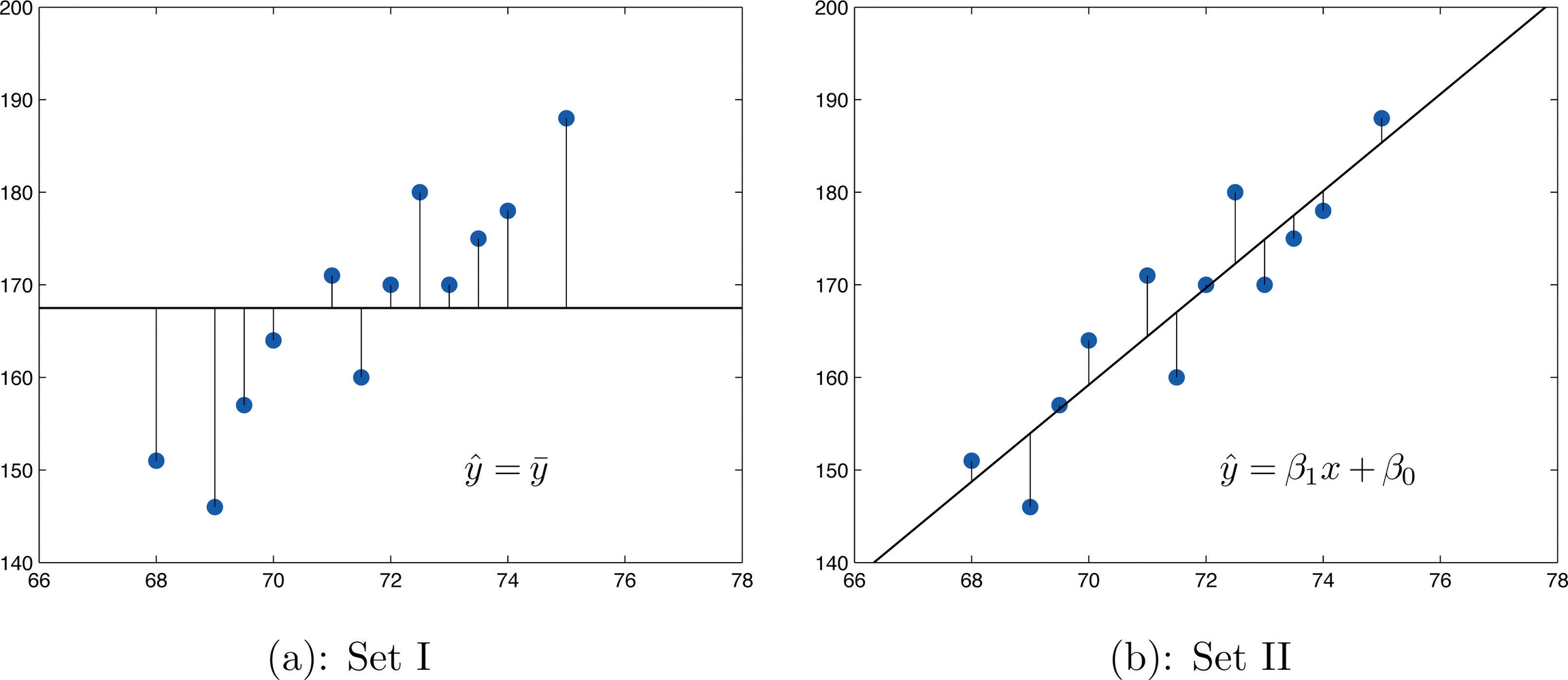
If the scatter diagram shows a linear trend upward or downward then it is useful to compute the least squares regression line $\hat{y}=\hat{β_1}x+\hat{β_0}$ and use it in predicting $y$.

Figure 10.12 "Same Scatter Diagram with Two Approximating Lines" illustrates this. In each panel we have plotted the height and weight data of Section 10.1 "Linear Relationships Between Variables".

This is the same scatter plot as Figure 10.2 "Plot of Height and Weight Pairs", with the average value line $\hat{y}= \bar{y}$ superimposed on it in the left panel and the least squares regression line imposed on it in the right panel. The errors are indicated graphically by the vertical line segments.

Figure 10.12 Same Scatter Diagram with Two Approximating Lines

The sum of the squared errors computed for the regression line, $SSE$ , is smaller than the sum of the squared errors computed for any other line. In particular it is less than the sum of the squared errors computed using the line $\hat{y}= \bar{y}$, which sum is actually the number $SS_{yy}$ that we have seen several times already. A measure of how useful it is to use the regression equation for prediction of $y$ is how much smaller $SSE$ is than $SS_{yy}$. In particular, the proportion of the sum of the squared errors for the line $\hat{y}= \bar{y}$ that is eliminated by going over to the least squares regression line is

$\frac{SS_{yy}−SSE} {SS_{yy}}= \frac{SS_{yy}}{SS_{yy}}−\frac{SSE} {SS_{yy}}=1−\frac{SSE}{ SS_{yy}}$

We can think of $\frac{SSE}{ SS_{yy}}$ as the proportion of the variability in $y$ that cannot be accounted for by the linear relationship between $x$ and $y$, since it is still there even when $x$ is taken into account in the best way possible (using the least squares regression line; remember that $SSE$ is the smallest the sum of the squared errors can be for any line).

Seen in this light, the coefficient of determination, the complementary proportion of the variability in $y$, is the proportion of the variability in all the $y$ measurements that is accounted for by the linear relationship between $x$ and $y$.

In the context of linear regression the coefficient of determination is always the square of the correlation coefficient $r$ discussed in Section 10.2 "The Linear Correlation Coefficient". Thus the coefficient of determination is denoted $r^2$, and we have two additional formulas for computing it.

The coefficient of determination of a collection of (x,y)(x,y) pairs is the number r2 computed by any of the following three expressions:

$r^2 = \frac{SS_{yy}−SSE} {SS_{yy}} = \frac{SS^2_{xy}}{ SS_{xx}SS_{yy}} = \hat{β_1} \frac{SS_{xy}}{SS_{yy}}$

It measures the proportion of the variability in y that is accounted for by the linear relationship between x and y.

If the correlation coefficient $r$ is already known then the coefficient of determination can be computed simply by squaring $r$, as the notation indicates, $r^2=(r)^2.$ .

EXAMPLE 10. The value of used vehicles of the make and model discussed in Note 10.19 "Example 3" in Section 10.4 "The Least Squares Regression Line" varies widely. The most expensive automobile in the sample in Table 10.3 "Data on Age and Value of Used Automobiles of a Specific Make and Model" has value $30,500, which is nearly half again as much as the least expensive one, which is worth $20,400. Find the proportion of the variability in value that is accounted for by the linear relationship between age and value.

[ Solution ]

The proportion of the variability in value $y$ that is accounted for by the linear relationship between it and age $x$ is given by the coefficient of determination, $r^2$ .

Since the correlation coefficient $r$ was already computed in Note 10.19 "Example 3" as $r = −0.819$, $r^2=(−0.819)^2=0.671$.

About 67% of the variability in the value of this vehicle can be explained by its age.

EXAMPLE 11. Use each of the three formulas for the coefficient of determination to compute its value for the example of ages and values of vehicles.

[ Solution ] In Note 10.19 "Example 3" in Section 10.4 "The Least Squares Regression Line" we computed the exact values

$SS_{xx}=14$, $SS_{xy}=-28.7$, $SS_{yy}=87.781$,  $\hat{β_1} = -2.05$

In Note 10.24 "Example 5" in Section 10.4 "The Least Squares Regression Line" we computed the exact value $SSE=28.946$

Inserting these values into the formulas in the definition, one after the other, gives

$r^2 = \frac{SS_{yy}−SSE} {SS_{yy}} = \frac{87.781−28.946}{87.781}=0.6702475479$ $r^2 = \frac{SS^2_{xy}}{ SS_{xx}SS_{yy}} =\frac{(−28.7)^2} {(14)(87.781)}=0.6702475479$ $r^2 = \hat{β_1} \frac{SS_{xy}}{SS_{yy}}= −2.05 \frac{(−28.7)}{87.781}=0.6702475479$ which rounds to 0.670.

The discrepancy between the value here and in the previous example is because a rounded value of $r$ from Note 10.19 "Example 3" was used there.

The actual value of $r$ before rounding is 0.8186864772, which when squared gives the value for $r^2$ obtained here.