6-3. The Sample Proportion

样本率/样本比例

1. Sample Proportion

Often sampling is done in order to estimate the proportion of a population that has a specific characteristic, such as the proportion of all items coming off an assembly line that are defective or the proportion of all people entering a retail store who make a purchase before leaving.

The population proportion is denoted p and the sample proportion is denoted $\hat{p}$ . Thus if in reality 43% of people entering a store make a purchase before leaving, p = 0.43; if in a sample of 200 people entering the store, 78 make a purchase, $\hat{p}$=78/200=0.39.

The sample proportion is a random variable: it varies from sample to sample in a way that cannot be predicted with certainty. Viewed as a random variable it will be written $\hat{P}$ . It has a mean and a standard deviation . Here are formulas for their values.

Suppose random samples of size n are drawn from a population in which the proportion with a characteristic of interest is p. The mean and standard deviation of the sample proportion $\hat{P}$ satisfy

  and  

where $q=1−p$ .

The Central Limit Theorem has an analogue for the population proportion $\hat{P}$. To see how, imagine that every element of the population that has the characteristic of interest is labeled with a 1, and that every element that does not is labeled with a 0. This gives a numerical population consisting entirely of zeros and ones. Clearly the proportion of the population with the special characteristic is the proportion of the numerical population that are ones; in symbols,

$p=\frac{number of 1s} {N}$

But of course the sum of all the zeros and ones is simply the number of ones, so the mean μ of the numerical population is

$μ=\frac{Σx}{N}=\frac{number of 1s}{N}$

Thus the population proportion p is the same as the mean μ of the corresponding population of zeros and ones. In the same way the sample proportion $\hat{p}$ is the same as the sample mean $\bar{x}$. Thus the Central Limit Theorem applies to$\hat{P}$. However, the condition that the sample be large is a little more complicated than just being of size at least 30.

2. The Sampling Distribution of the Sample Proportion

For large samples, the sample proportion is approximately normally distributed,

with mean

and standard deviation

A sample is large if the interval lies wholly within the interval $[0,1]$ .

In actual practice p is not known, hence neither is . In that case in order to check that the sample is sufficiently large we substitute the known quantity $\hat{p}$ for $p$ . This means checking that the interval

$[ \hat{p} - 3 \sqrt{\frac{\hat{p}(1-\hat{p}) } {n } }, \space \space \space \hat{p} + 3 \sqrt{\frac{\hat{p}(1-\hat{p}) } {n } }]$

lies wholly within the interval $[0,1]$. This is illustrated in the examples.

Figure "Distribution of Sample Proportions" shows that when p = 0.1 a sample of size 15 is too small but a sample of size 100 is acceptable.

Distribution of Sample Proportions

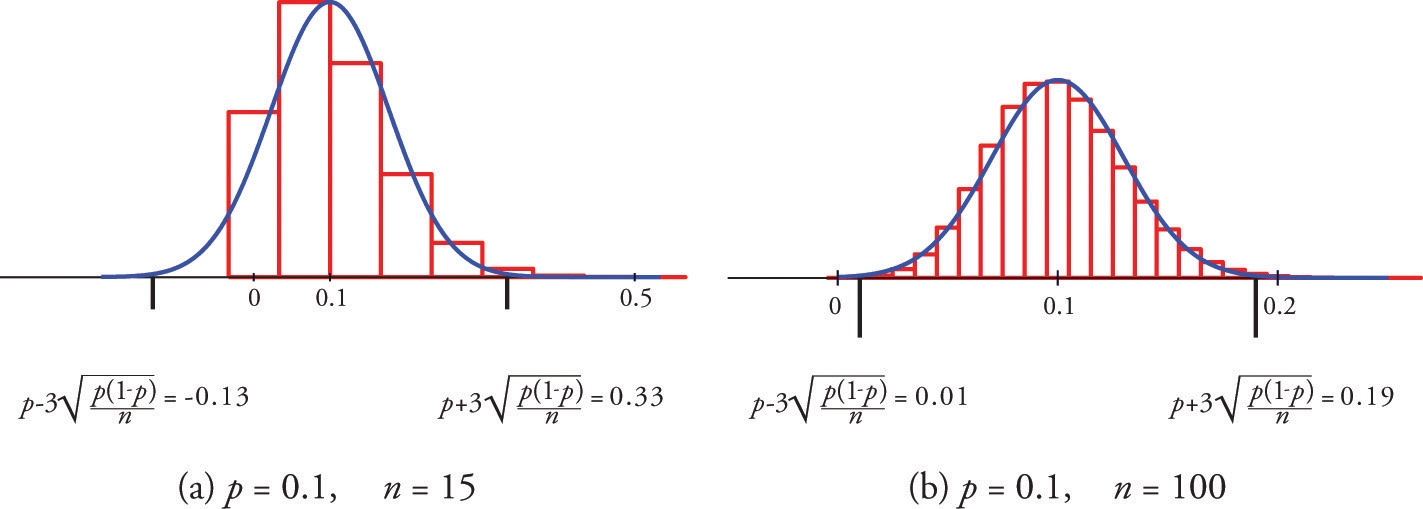
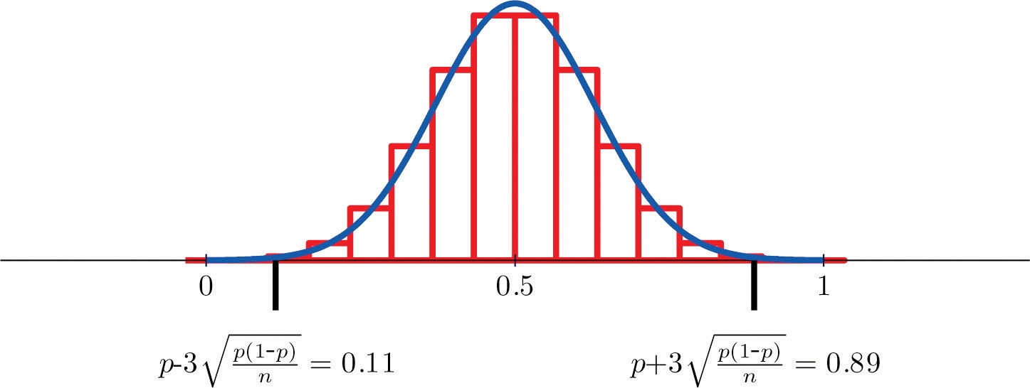
Figure "Distribution of Sample Proportions for " shows that when p = 0.5 a sample of size 15 is acceptable.

Distribution of Sample Proportions for p = 0.5 and n = 15

EXAMPLE 7. Suppose that in a population of voters in a certain region 38% are in favor of particular bond issue. Nine hundred randomly selected voters are asked if they favor the bond issue.

1. Verify that the sample proportion $\hat{P}$ computed from samples of size 900 meets the condition that its sampling distribution be approximately normal.

2. Find the probability that the sample proportion computed from a sample of size 900 will be within 5 percentage points of the true population proportion.

[ Solution ]

1.  and   Then so  which lies wholly within the interval [0,1], so it is safe to assume that $\hat{P}$ is approximately normally distributed.

2. $P(0.33<\hat{P}<0.43)$ $=P(−3.09<Z<3.09)$ $=P(3.09)−P(−3.09)$ $=0.9990−0.0010=0.9980$

R Source

library(Rstat)

# 2.
mu <- 0.38; 
n <- 900; sig <- sqrt(mu * (1-mu) / n)
sig
 
a <- 0.33;  b <- 0.43
norm.trans(mu, sig, a, b)

2. Probability

> # 2.
> mu <- 0.38; 
> n <- 900; sig <- sqrt(mu * (1-mu) / n)
> sig
## [1] 0.01617955
>  
> a <- 0.33;  b <- 0.43
> norm.trans(mu, sig, a, b)
## Pr(0.33 < X < 0.43) =  0.9980006 
## Pr(-3.0903 < Z < 3.0903) =  0.9980006 

2-Plot

EXAMPLE 8. An online retailer claims that 90% of all orders are shipped within 12 hours of being received. A consumer group placed 121 orders of different sizes and at different times of day; 102 orders were shipped within 12 hours.

1. Compute the sample proportion of items shipped within 12 hours.

2. Confirm that the sample is large enough to assume that the sample proportion is normally distributed. Use p = 0.90, corresponding to the assumption that the retailer’s claim is valid.

3. Assuming the retailer’s claim is true, find the probability that a sample of size 121 would produce a sample proportion so low as was observed in this sample.

4. Based on the answer to part (3), draw a conclusion about the retailer’s claim.

[ Solution ]

1. $\hat{p} = \frac{x}{n} =\frac{102}{121} = 0.84$

2. $[0.82, 0.98]⊂[0,1]$

3. $P(\hat{P}≤0.84)$ $=P(Z≤\frac{0.84−0.90} {0.027})$ $=P(Z≤−2.20)=0.0139$

R Source

library(Rstat)

# 1. 

# 2.
mu <- 0.90; 
n <- 121; sig <- sqrt(mu * (1-mu) / n)
sig
 
a <- 0;  b <- 0.84
norm.trans(mu, sig, a, b)

2. Probability

> mu <- 0.90; 
> n <- 121; sig <- sqrt(mu * (1-mu) / n)
> sig
## [1] 0.02727273
>  
> a <- 0;  b <- 0.84
> norm.trans(mu, sig, a, b)
## Pr(0 < X < 0.84) =  0.01390345 
## Pr(-33 < Z < -2.2) =  0.01390345 

2-Plot

样本率/样本比例 sample proportion