11-2. Chi-Square One-Sample Goodness-of-Fit Tests

Suppose we wish to determine if an ordinary-looking six-sided die is fair, or balanced, meaning that every face has probability 1/6 of landing on top when the die is tossed. We could toss the die dozens, maybe hundreds, of times and compare the actual number of times each face landed on top to the expected number, which would be 1/6 of the total number of tosses. We wouldn’t expect each number to be exactly 1/6 of the total, but it should be close. To be specific, suppose the die is tossed n = 60 times with the results summarized in Table 11.8 "Die Contingency Table". For ease of reference we add a column of expected frequencies, which in this simple example is simply a column of 10s. The result is shown as Table 11.9 "Updated Die Contingency Table". In analogy with the previous section we call this an “updated” table. A measure of how much the data deviate from what we would expect to see if the die really were fair is the sum of the squares of the differences between the observed frequency O and the expected frequency E in each row, or, standardizing by dividing each square by the expected number, the sum $Σ(O−E)^2/E$ . If we formulate the investigation as a test of hypotheses, the test is

$H_0 : The die is fair$ vs. $H_a: The die is not fair$

Table 11.8 Die Contingency Table

Die Value	Assumed Distribution	Observed Frequency
1	1/6	9
2	1/6	15
3	1/6	9
4	1/6	8
5	1/6	6
6	1/6	13

Table 11.9 Updated Die Contingency Table

Die Value	Assumed Distribution	Observed Freq.	Expected Freq.
1	1/6	9	10
2	1/6	15	10
3	1/6	9	10
4	1/6	8	10
5	1/6	6	10
6	1/6	13	10

We would reject the null hypothesis that the die is fair only if the number $Σ(O−E)^2/E$ is large, so the test is right-tailed. In this example the random variable $Σ(O−E)^2/E$ has the chi-square distribution with five degrees of freedom.

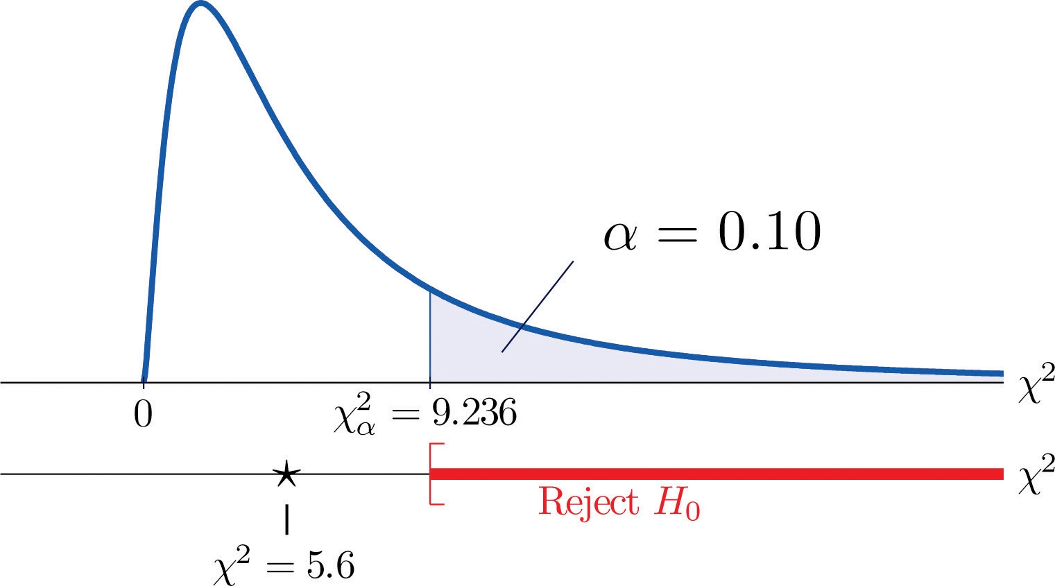
If we had decided at the outset to test at the 10% level of significance, the critical value defining the rejection region would be, reading from Figure 12.4 "Critical Values of Chi-Square Distributions", $χ^2_α=χ^2_{0.10}=9.2366$ , so that the rejection region would be the interval $[9.236,∞)$ .

When we compute the value of the standardized test statistic using the numbers in the last two columns of Table 11.9 "Updated Die Contingency Table", we obtain

$Σ(O−E)^2/E$ $= \frac{(−1)^2} {10}+\frac{5^2} {10}+\frac{(−1)^2} {10}+\frac{(−2)^2} {10}+\frac{(−4)^2} {10}+\frac{3^2} {10}$ $=0.1+2.5+0.1+0.4+1.6+0.9=5.6$

Since 5.6 < 9.236 the decision is not to reject $H_0$ . See Figure 11.5 "Balanced Die". The data do not provide sufficient evidence, at the 10% level of significance, to conclude that the die is loaded.

Figure 11.5 Balanced Die

library(Rstat)

# basic function : chisq.test(x)

x <- c(9, 15, 9, 8, 6, 13)
alpha <- 0.10

ct <- chisq.test(x); ct

# Graph of Chi-square Test : chitest.plot2()
chitest.plot2(stat=ct$stat, df=ct$para, alp=alpha, side="up")

> ct <- chisq.test(x); ct
##
##         Chi-squared test for given probabilities
## 
## data:  x
## X-squared = 5.6, df = 5, p-value = 0.3471
## 
>

> chitest.plot2(stat=ct$stat, df=ct$para, alp=alpha, side="up")
## P-v = 0.3471

In the general situation we consider a discrete random variable that can take I different values, $x_1,x_2,…,x_I$ for which the default assumption is that the probability distribution is $x$ $x_1$ $x_2$ $…$ $x_I$ $P(x)$ $p_1$ $p_2$ $…$ $p_I$

We wish to test the hypotheses

$H_0:The assumed probability distribution for X is valid$ vs. $H_a:The assumed probability distribution for X is not valid$

We take a sample of size n and obtain a list of observed frequencies. This is shown in Table 11.10 "General Contingency Table". Based on the assumed probability distribution we also have a list of assumed frequencies, each of which is defined and computed by the formula

$E_i=n×p_i$

Table 11.10 General Contingency Table

Factor Levels

Assumed Distribution

Observed Frequency

⋮

Table 11.10 "General Contingency Table" is updated to Table 11.11 "Updated General Contingency Table" by adding the expected frequency for each value of X. To simplify the notation we drop indices for the observed and expected frequencies and represent Table 11.11 "Updated General Contingency Table" by Table 11.12 "Simplified Updated General Contingency Table".

Table 11.11 Updated General Contingency Table

Factor Levels

Assumed Distribution

Observed Freq.

Expected Freq.

⋮

Table 11.12 Simplified Updated General Contingency Table

Factor Levels

Assumed Distribution

Observed Freq.

Expected Freq.

⋮

Here is the test statistic for the general hypothesis based on Table 11.12 "Simplified Updated General Contingency Table", together with the conditions that it follow a chi-square distribution.

Test Statistic for Testing Goodness of Fit to a Discrete Probability Distribution
$χ^2=\frac{Σ(O−E)^2} {E}$
where the sum is over all the rows of the table (one for each value of X).
If
the true probability distribution of $X$ is as assumed, and
the observed count O of each cell in Table 11.12 "Simplified Updated General Contingency Table" is at least 5,
then $χ^2$ approximately follows a chi-square distribution with $df=(I−1)$ degrees of freedom.

The test is known as a goodness-of-fit $χ^2$ test since it tests the null hypothesis that the sample fits the assumed probability distribution well. It is always right-tailed, since deviation from the assumed probability distribution corresponds to large values of $χ^2$ .

Testing is done using either of the usual five-step procedures.

EXAMPLE 2. Table 11.13 "Ethnic Groups in the Census Year" shows the distribution of various ethnic groups in the population of a particular state based on a decennial U.S. census. Five years later a random sample of 2,500 residents of the state was taken, with the results given in Table 11.14 "Sample Data Five Years After the Census Year" (along with the probability distribution from the census year). Test, at the 1% level of significance, whether there is sufficient evidence in the sample to conclude that the distribution of ethnic groups in this state five years after the census had changed from that in the census year.

TABLE 11.13 ETHNIC GROUPS IN THE CENSUS YEAR

Ethnicity	White	Black	Amer.-Indian	Hispanic	Asian	Others
Proportion	0.743	0.216	0.012	0.012	0.008	0.009

TABLE 11.14 SAMPLE DATA FIVE YEARS AFTER THE CENSUS YEAR

Ethnicity	Assumed Distribution	Observed Frequency
White	0.743	1732
Black	0.216	538
American-Indian	0.012	32
Hispanic	0.012	42
Asian	0.008	133
Others	0.009	23

[ Solution ]

We test using the critical value approach.

Step 1. The hypotheses of interest in this case can be expressed as $H_0:The distribution of ethnic groups has not changed$
vs. $H_a:The distribution of ethnic groups has changed$
Step 2. The distribution is chi-square.
Step 3. To compute the value of the test statistic we must first compute the expected number for each row of Table 11.14 "Sample Data Five Years After the Census Year". Since n = 2500, using the formula $E_i=n×p_i$ and the values of pi from either Table 11.13 "Ethnic Groups in the Census Year" or Table 11.14 "Sample Data Five Years After the Census Year", $E_1=2500×0.743=1857.5$ $E_2=2500×0.216=540$ $E_3=2500×0.012=30$ $E_4=2500×0.012=30$ $E_5=2500×0.008=20$ $E_6=2500×0.009=22.5$
Table 11.14 "Sample Data Five Years After the Census Year" is updated to Table 11.15 "Observed and Expected Frequencies Five Years After the Census Year".
TABLE 11.15 OBSERVED AND EXPECTED FREQUENCIES FIVE YEARS AFTER THE CENSUS YEAR
Ethnicity
Assumed Dist.
Observed Freq.
Expected Freq.
White
0.743
1732
1857.5
Black
0.216
538
540
American-Indian
0.012
32
30
Hispanic
0.012
42
30
Asian
0.008
133
20
Others
0.009
23
22.5
The value of the test statistic is $χ^2$ $= Σ(O−E)^2/E$ $=\frac{(1732−1857.5)^2} {1857.5} +\frac{(538−540)^2}{540} + \frac{(32−30)^2}{30}$ $+ \frac{(42−30)^2}{30} + \frac{(133−20)^2}{20} + \frac{(23−22.5)^2}{22.5}$ $=651.881$
Since the random variable takes six values, I = 6. Thus the test statistic follows the chi-square distribution with $df=(6−1)=5$ degrees of freedom.
Since the test is right-tailed, the critical value is $χ_{0.01}^2$ . Reading from Figure 12.4 "Critical Values of Chi-Square Distributions", $χ_{0.01}^2=15.086$ , so the rejection region is $[15.086,∞)$ .
Since $651.881 > 15.086$ the decision is to reject the null hypothesis. See Figure 11.6. The data provide sufficient evidence, at the 1% level of significance, to conclude that the ethnic distribution in this state has changed in the five years since the U.S. census.

Figure 11.6 Note 11.15 "Example 2"

library(Rstat)

x <- c(1732, 538, 32, 42, 133, 23)
p <- c(0.743, 0.216, 0.012, 0.012, 0.008, 0.009)
alpha <- 0.01

# Chi-square Test
ct <- chisq.test(x, p=p); ct

# Graph of Chi-square Test : chitest.plot2()
chitest.plot2(stat=ct$stat, df=ct$para, alp=alpha, side="up", pup=0.99999)

> ct <- chisq.test(x, p=p); ct
## 
##         Chi-squared test for given probabilities
## 
## data:  x
## X-squared = 651.88, df = 5, p-value < 2.2e-16

$χ^2 = 651.881$ > $χ_{0.01}^2=15.086$

> chitest.plot2(stat=ct$stat, df=ct$para, alp=alpha, side="up", pup=0.99999)
## P-v = 0

Previous11-1. Exercises Next11-2. Exercises

Last updated 4 years ago

Ethnicity	Assumed Dist.	Observed Freq.	Expected Freq.
White	0.743	1732	1857.5
Black	0.216	538	540
American-Indian	0.012	32	30
Hispanic	0.012	42	30
Asian	0.008	133	20
Others	0.009	23	22.5