8-5. Large Sample Tests for a Population Proportion

Both the critical value approach and the p-value approach can be applied to test hypotheses about a population proportion $p$ .

The null hypothesis will have the form $H_0:p=p_0$ for some specific number $p_0$ between 0 and 1.

The alternative hypothesis will be one of the three inequalities $p<p_0, p>p_0, or \space p≠p_0$ for the same number $p_0$ that appears in the null hypothesis.

The information in Section 6.3 "The Sample Proportion" in Chapter 6 "Sampling Distributions" gives the following formula for the test statistic and its distribution.

In the formula $p_0$ is the numerical value of $p$ that appears in the two hypotheses, $q_0=1−p_0, \hat{p}$ is the sample proportion, and $n$ is the sample size. Remember that the condition that the sample be large is not that $n$ be at least 30 but that the interval

lie wholly within the interval $[0,1].$

Standardized Test Statistic for Large Sample Hypothesis Tests Concerning a Single Population Proportion

$z_o = \frac{\hat p - p_0}{ \sqrt{\frac{p_0 q_0}{n} }}$

The test statistic has the standard normal distribution.

The distribution of the standardized test statistic and the corresponding rejection region for each form of the alternative hypothesis (left-tailed, right-tailed, or two-tailed), is shown in Figure 8.14 "Distribution of the Standardized Test Statistic and the Rejection Region".

Figure 8.14 Distribution of the Standardized Test Statistic and the Rejection Region

EXAMPLE 12. A soft drink maker claims that a majority of adults prefer its leading beverage over that of its main competitor’s. To test this claim 500 randomly selected people were given the two beverages in random order to taste. Among them, 270 preferred the soft drink maker’s brand, 211 preferred the competitor’s brand, and 19 could not make up their minds. Determine whether there is sufficient evidence, at the 5% level of significance, to support the soft drink maker’s claim against the default that the population is evenly split in its preference.

[ Solution ]

We must check that the sample is sufficiently large to validly perform the test. Since

$\hat{p} = \frac {270}{500} = 0.54,$

$\sqrt{ \frac{ \hat{p} (1-\hat{p}) }{n} } = \sqrt{ \frac { (0.54)(0.46) }{ 500}} ≈ 0.02$

hence,

$[ \hat {p} - 3 \sqrt{ \frac{ \hat{p} (1-\hat{p}) }{n} }, \hat{p} + \sqrt{ \frac{ \hat{p} (1-\hat{p}) }{n} }]$

$= [0.54 - 3 (0.02), 0.54 + 3 (0.02)]$

$= [0.48, 0.60] ⊂[0,1]$

so the sample is sufficiently large.

• Step 1. The relevant test is $H_0:p=0.50 vs. Ha:p>0.50, @ α=0.05$

  where p denotes the proportion of all adults who prefer the company’s beverage over that of its competitor’s beverage.

• Step 2. The test statistic is $z_o= (\hat{p}−p_0) / \sqrt{ \frac {p_0 q_0} {n} }$

  and has the standard normal distribution.

• Step 3. The value of the test statistic is $z_o= \frac {(\hat{p}−p_0)} { \sqrt{ \frac {p_0 q_0} {n} } }= \frac {(0.54 - 0.50) } { \sqrt { \frac {(0.5) (0.5)}{500}}} = 1.789$

• Step 4. Since the symbol in $H_a$ is “ $>$ ” this is a right-tailed test, so there is a single critical value, $z_α=z_{0.05}.$ Reading from the last line in Figure 12.3 "Critical Values of " its value is 1.645. The rejection region is $[1.645,∞).$

• Step 5. the test statistic falls in the rejection region. The decision is to reject $H_0$ .

• In the context of the problem our conclusion is:

  The data provide sufficient evidence, at the 5% level of significance, to conclude that a majority of adults prefer the company’s beverage to that of their competitor’s.

Figure 8.15 Rejection Region and Test Statistic for Note 8.47 "Example 12"

R Source

n <- 500                  # number of samples
xb <- 270
p0 <- 0.5
alpha <- 0.05             # 

# in case of right-tail test
pb <- xb / n               # sample proportion
se <- sqrt(p*(1-p)/n)     # std of sample proportion

z_c <- qnorm(1-alpha); z_c
z_o <- (pb - p0)/se; z_o

if (z_o >= z_c)  cat("Reject Ho.\n") else 
                 cat ("Can not reject Ho.\n")

Result

> z_c <- qnorm(1-alpha); z_c
## [1] 1.644854
> z_o <- (pb - p0)/se; z_o
## [1] 1.809325
> 
> if (z_o >= z_c)  cat("Reject Ho.\n") else 
+                  cat ("Can not reject Ho.\n")
## Reject Ho.

EXAMPLE 13. Globally the long-term proportion of newborns who are male is 51.46%. A researcher believes that the proportion of boys at birth changes under severe economic conditions. To test this belief randomly selected birth records of 5,000 babies born during a period of economic recession were examined. It was found in the sample that 52.55% of the newborns were boys. Determine whether there is sufficient evidence, at the 10% level of significance, to support the researcher’s belief.

[ Solution ]

$\sqrt{ \frac{ \hat{p} (1-\hat{p}) }{n} } = \sqrt{ \frac { (0.5255)(0.4745) }{ 5000}} ≈ 0.01$

hence,

$[ \hat {p} - 3 \sqrt{ \frac{ \hat{p} (1-\hat{p}) }{n} }, \hat{p} + \sqrt{ \frac{ \hat{p} (1-\hat{p}) }{n} }]$

$= [0.5225 - 3 (0.01), 0.5225 + 3 (0.01)]$

$= [0.4925, 0.5555] ⊂[0,1]$

• Step 1. the hypothesis test is $H0:p=0.5146 vs. Ha:p=≠0.5146, @ α=0.10$

• Step 2. The test statistic is $z_o= \frac {(\hat{p}−p_0)} { \sqrt{ \frac {p_0 q_0} {n} } }$

  and has the standard normal distribution.

• Step 3. The value of the test statistic is $z_o= \frac {(\hat{p}−p_0)} { \sqrt{ \frac {p_0 q_0} {n} } } = \frac {(0.5255− 0.5146)} { \sqrt{ \frac {(0.5146)(0.4854)} {5000} } } ≈ 1.542$

• Step 4. Since the symbol in $H_a$ is “ $≠$ ” this is a two-tailed test, so there are a pair of critical values, $±z_{α∕2}=±z_{0.05}=±1.645.$ The rejection region is $(−∞,−1.645]∪[1.645,∞).$

• Step 5. the test statistic does not fall in the rejection region. The decision is not to reject $H_0$ .

• In the context of the problem our conclusion is:

  The data do not provide sufficient evidence, at the 10% level of significance, to conclude that the proportion of newborns who are male differs from the historic proportion in times of economic recession.

Figure 8.16 Rejection Region and Test Statistic for Note 8.48 "Example 13"

R Source

n <- 5000                  # number of samples
xb <- 2625
p0 <- 0.5146
alpha <- 0.10              # 

# in case of two-tail test
pb <- xb / n               # sample proportion
se <- sqrt(p*(1-p)/n)     # std of sample proportion

z_c <- qnorm(1-alpha/2); z_c
z_o <- (pb - p0)/se; z_o

if (z_o <= -z_c || z_o >= z_c ) cat("Reject Ho.\n") else 
                                cat ("Can not reject Ho.\n")

Result

> z_c <- qnorm(1-alpha/2); z_c
## [1] 1.644854
> z_o <- (pb - p0)/se; z_o
## [1] 1.487613
> 
> if (z_o <= -z_c || z_o >= z_c ) cat("Reject Ho.\n") else 
+                                 cat ("Can not reject Ho.\n")
## Can not reject Ho.

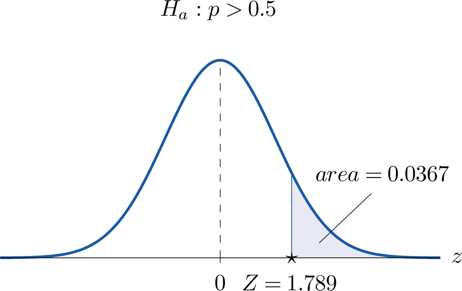
EXAMPLE 14. Perform the test of Note 8.47 "Example 12" using the p-value approach.

[ Solution ]

We already know that the sample size is sufficiently large to validly perform the test.

• Steps 1–3 of the five-step procedure described in Section 8.3.2 "The " have already been done in Note 8.47 "Example 12" so we will not repeat them here, but only say that we know that the test is right-tailed and that value of the test statistic is $Z = 1.789.$

• Step 4. Since the test is right-tailed the p-value is the area under the standard normal curve cut off by the observed test statistic, z = 1.789, and therefore the p-value is $(1−0.9633)=0.0367.$

• Step 5. Since the p-value is less than $α=0.05$ , the decision is to reject $H_0$ .

Figure 8.17 P-Value for Note 8.49 "Example 14"

• Using Rstat Package : bntest2.plot()

R Source

library(Rstat)

bntest2.plot(x=270, n=500, p0=0.5, alp=0.05, side="up")

Result

> bntest2.plot(x=270, n=500, p0=0.5, alp=0.05, side="up")
## Exact Binomial Test:     x/n = 0.54      P-v = P(X ≥ 270) = 0.0405 
## Normal approximation:    Z0 = 1.7889     P-v = P(Z > Z0) = 0.0368 
## Continuity correction:   Z0 = 1.7441     P-v = P(Z > Z0) = 0.0406 

Plot

[Decision Rule]

• p-value=0.0368 => if p-value is less than alpha(=0.05), reject Ho. Otherwise, Can not reject Ho.

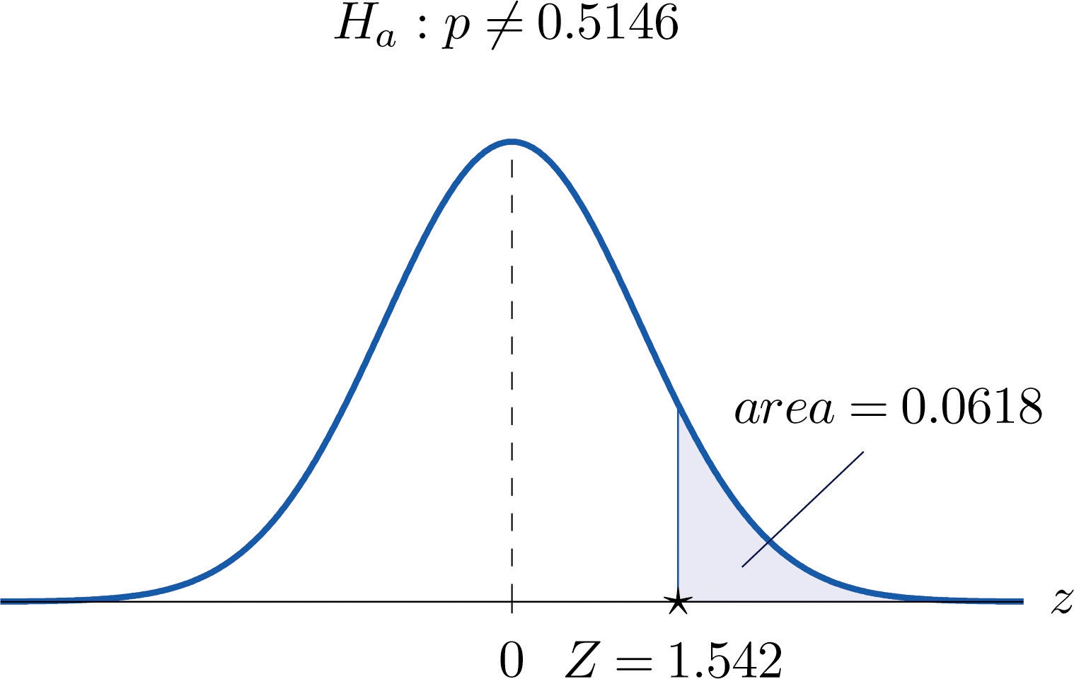
EXAMPLE 15. Perform the test of Note 8.48 "Example 13" using the p-value approach.

[ Solution ]

We already know that the sample size is sufficiently large to validly perform the test.

• Steps 1–3 of the five-step procedure described in Section 8.3.2 "The " have already been done in Note 8.48 "Example 13". They tell us that the test is two-tailed and that value of the test statistic is $z = 1.542.$

• Step 4. Since the test is two-tailed the p-value is the double of the area under the standard normal curve cut off by the observed test statistic, $z = 1.542.$

  By Figure 12.2 "Cumulative Normal Probability" that area is $(1−0.9382)=0.0618$ as illustrated in Figure 8.18, hence the p-value is $2×0.0618=0.1236.$

• Step 5. Since the p-value is greater than $α=0.10$ the decision is not to reject $H_0$ .

Figure 8.18 P-Value for Note 8.50 "Example 15"

• Using Rstat Package : bntest2.plot()

R Source

library(Rstat)

bntest2.plot(x=2625, n=5000, p0=0.5146, alp=0.10, side="two")

Result

> bntest2.plot(x=2625, n=5000, p0=0.5146, alp=0.10, side="two")
## Exact Binomial Test:     x/n = 0.525     P-v = Σ[f(y) ≤ f(2625)] = 0.145 
## Normal approximation:    Z0 = 1.4714     P-v = 2×P(Z > |Z0|) = 0.1412 
## Continuity correction:   Z0 = 1.4573     P-v = 2×P(Z > |Z0|) = 0.145 

Plot

[Decision Rule]

• p-value=0.1412 => if p-value is less than alpha(=0.10), reject Ho. Otherwise, Can not reject Ho.