3-1. Sample Spaces, Events, and Their Probabilities

样本空间和事件和概率

样本空间和事件 (概率论) - 文氏图(Venn Diagram) - 树形图（Tree Diagram）
概率（Probability）

1. Sample Spaces and Events

A random experiment is a mechanism that produces a definite outcome that cannot be predicted with certainty. The sample space associated with a random experiment is the set of all possible outcomes. An event is a subset of the sample space.

An event E is said to occur on a particular trial of the experiment if the outcome observed is an element of the set E.

EXAMPLE 1. Construct a sample space for the experiment that consists of tossing a single coin.

[ Solution ] $S = \{ H, T \}$

# install.packages("prob")
library(prob)

tosscoin(1)

> tosscoin(1)
##   toss1
## 1     H
## 2     T

EXAMPLE 2. Construct a sample space for the experiment that consists of rolling a single die. Find the events that correspond to the phrases “an even number is rolled” and “a number greater than two is rolled.”

[ Solution ] $S = \{ 1, 2, 3, 4, 5, 6 \}$ , $E_1 = \{ 2, 4, 6\}$ , $E_2 = \{ 3, 4, 5, 6 \}$

library(prob)

## 1. Sample Space : rolling a single die
rolldie(1)

# 2. Event 1 : an even number is rolled
S <- rolldie(1)
E1 <- subset(S, X1 %% 2 ==0); E1

# 3. Event 2 : a number greater than two is rolled.
S <- rolldie(1)
E2 <- subset(S, X1 > 2); E2

> # 1. Sample Space : rolling a single die
> rolldie(1)
##   X1
## 1  1
## 2  2
## 3  3
## 4  4
## 5  5
## 6  6
##

> # 2. Event1 : an even number is rolled
> S <- rolldie(1)
> E1 <- subset(S, X1 %% 2 ==0); E1
##   X1
## 2  2
## 4  4
## 6  6

> # 3. Event 2 : a number greater than two is rolled.
> S <- rolldie(1)
> E2 <- subset(S, X1 > 2); E2
##   X1
## 3  3
## 4  4
## 5  5
## 6  6

1-1. Venn Diagram

A graphical representation of a sample space and events is a Venn diagram

EXAMPLE 3. A random experiment consists of tossing two coins.

Construct a sample space for the situation that the coins are indistinguishable, such as two brand new pennies.
Construct a sample space for the situation that the coins are distinguishable, such as one a penny and the other a nickel.

[ Solution ]

two same coins : two head -> 2h, two tails -> 2t, 2 different faces : d => $S = \{ 2h, 2t, d \}$
two different coins (penny, nickel) : $S = \{ hh, th, ht, tt\}$

1-2. Venn Diagram Plot in R

type of count data.

A   450
B   1800
A and B both    230

I want to develop a colorful (possibly semi-transparency at intersections) like the following Venn diagram.

require(venneuler)
v <- venneuler(c(A=450, B=1800, "A&B"=230))
plot(v)

# install package
if (!requireNamespace("BiocManager", quietly = TRUE))
    install.packages("BiocManager")
BiocManager::install("VennDiagram")
library("VennDiagram")

# 2-set diagram
venn.plot <- draw.pairwise.venn(30, 20, 10, c("A-up", "B-up"), scaled = FALSE);

venn.plot <- draw.triple.venn(
  area1 = 60,
  area2 = 70,
  area3 = 80,
  n12 = 30,
  n23 = 20,
  n13 = 10,
  n123 = 5,
  category = c("A_up-regulation", "B_up-regulation", "C_up-  regulation"),
);

# 3-set diagram
venn.plot <- draw.triple.venn(
  area1 = 60,
  area2 = 70,
  area3 = 80,
  n12 = 30,
  n23 = 20,
  n13 = 10,
  n123 = 5,
  category = c("A_up-regulation", "B_up-regulation", "C_up-  regulation"),
);

# 4-set diagram
venn.plot <- draw.quad.venn(
  area1 = 90,
  area2 = 80,
  area3 = 75,
  area4 = 49,
  n12 = 37,
  n13 = 25,
  n14 = 26,
  n23 = 34,
  n24 = 30,
  n34 = 22,
  n123 = 16,
  n124 = 15,
  n134 = 10,
  n234 = 12,
  n1234 = 3,
  category = c("First", "Second", "Third", "Fourth"),
  fill = c("orange", "red", "green", "blue"),
  lty = "dashed",
  cex = 2,
  cat.cex=2,
  cat.col = c("orange", "red", "green", "blue")
);

[ 참고자료 - Venn Diagram ]

1-3. tree diagram

A device that can be helpful in identifying all possible outcomes of a random experiment, particularly one that can be viewed as proceeding in stages, is what is called a tree diagram.

EXAMPLE 4. Construct a sample space that describes all three-child families according to the genders of the children with respect to birth order.

[ Solution ] $S = \{ bbb, bbg, bgb, bgg, gbb, gbg, ggb, ggg \}$ , g=girl ; b=boy

The line segments are called branches of the tree. The right ending point of each branch is called a node. The nodes on the extreme right are the final nodes; to each one there corresponds an outcome, as shown in the figure.

1-4. Tree Diagram in R

fancyRpartPlot in R

How to create a massive tree diagram in RStudio?

Introduction to data.tree

PROBABILITY TREE DIAGRAMS IN R

venn.diagram From VennDiagram v1.6.20 by Paul Boutros

2. Probability

The probability of an outcome e in a sample space S is a number p between 0 and 1 that measures the likelihood that e will occur on a single trial of the corresponding random experiment. The value $p = 0$ corresponds to the outcome e being impossible and the value $p = 1$ corresponds to the outcome e being certain.

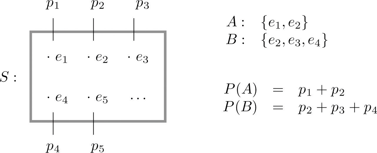
The probability of an event A is the sum of the probabilities of the individual outcomes of which it is composed. It is denoted $p(A)$ .

If an event $E$ is $E = \{e_1, e_2, ..., e_k \}$ , then
$P(E)=P(e_1)+P(e_2)+ ⋅ ⋅ ⋅ +P(e_k)$

EXAMPLE 5. A coin is called “balanced” or “fair” if each side is equally likely to land up. Assign a probability to each outcome in the sample space for the experiment that consists of tossing a single fair coin.

[ Solution ] $S = \{ H, T \}$ , $P(H) = P(T) =1/2$

# install.packages("prob")
library(prob)

tosscoin(1, makespace = TRUE)

> tosscoin(1, makespace = TRUE)
##   toss1 probs
## 1     H   0.5
## 2     T   0.5

EXAMPLE 6. A die is called “balanced” or “fair” if each side is equally likely to land on top. Assign a probability to each outcome in the sample space for the experiment that consists of tossing a single fair die. Find the probabilities of the events $E$ : “an even number is rolled” and $T$ : “a number greater than two is rolled.”

[ Solution ] $S = \{ 1, 2, 3, 4, 5, 6 \}$

$E = \{ 2, 4, 6\}$ , $P(E) = 3 / 6 = 1/2$
$T = \{3, 4, 5, 6 \}$ , $P(T) = 4/6 = 2/3$

library(prob)

# 1. Sample Space
S <- rolldie(1, makespace = TRUE); S

# 2. P(E)
E <- subset(S, X1 %% 2 == 0); E
Prob(S, X1 %% 2 == 0)    # or Prob(E)

# 3. P(T)
T <- subset(S, X1 > 2); T
Prob(S, X1 > 2)          # or Prob(T)

> # 1. Sample Space
> S <- rolldie(1, makespace = TRUE); S
##   X1     probs
## 1  1 0.1666667
## 2  2 0.1666667
## 3  3 0.1666667
## 4  4 0.1666667
## 5  5 0.1666667
## 6  6 0.1666667

> # 2. P(E)
> E <- subset(S, X1 %% 2 == 0); E
##   X1     probs
## 2  2 0.1666667
## 4  4 0.1666667
## 6  6 0.1666667
> Prob(S, X1 %% 2 == 0)    # or Prob(E)
## [1] 0.5

> # 3. P(T)
> T <- subset(S, X1 > 2); T
##   X1     probs
## 3  3 0.1666667
## 4  4 0.1666667
## 5  5 0.1666667
## 6  6 0.1666667
> Prob(S, X1 > 2)          # or Prob(T)
## [1] 0.6666667

EXAMPLE 7. Two fair coins are tossed. Find the probability that the coins match, i.e., either both land heads or both land tails.

[ Solution ]

identical coins : $S = \{ 2h, 2t, d \}$ , $E = \{2h, 2t \}$ => $P(E) = 2/3$
two different coins : $S^t = \{ 2h, ht, th, 2t \}$ , $E^t = \{2h, 2t \}$ => $P(E^t) = 2/4 = 1/2$

[ Solution 1 ]

library(prob)

a <- tosscoin(2, makespace = TRUE); a

S1 <- subset(a, toss1 == toss2); S1
S2 <- subset(a, toss1 != toss2); S2

S2[,1] <- "D" ; S2
S2[,2] <- "D" ; S2

# 1) Sample Space
S <- union(S1, S2)
S$probs <- 1/3; S

# 2) Probability that the coins match..
Prob(S, toss1 == "H" | toss2 =="T")

> a <- tosscoin(2, makespace = TRUE); a
##   toss1 toss2 probs
## 1     H     H  0.25
## 2     T     H  0.25
## 3     H     T  0.25
## 4     T     T  0.25
> 
> S1 <- subset(a, toss1 == toss2); S1
##   toss1 toss2 probs
## 1     H     H  0.25
## 4     T     T  0.25
> S2 <- subset(a, toss1 != toss2); S2
##   toss1 toss2 probs
## 2     T     H  0.25
## 3     H     T  0.25
>
> S2[,1] <- "D" ; S2
##   toss1 toss2 probs
## 2     D     H  0.25
## 3     D     T  0.25
> S2[,2] <- "D" ; S2
##   toss1 toss2 probs
## 2     D     D  0.25
## 3     D     D  0.25

> # 1) Sample Space
> S <- union(S1, S2); S
##   toss1 toss2 probs
## 1     H     H  0.25
## 2     D     D  0.25
## 4     T     T  0.25
> 
> S$probs <- 1/3; S
##   toss1 toss2     probs
## 1     H     H 0.3333333
## 2     D     D 0.3333333
## 4     T     T 0.3333333
> Prob(S, toss1 == "H" | toss2 =="T")
## [1] 0.6666667

> # 2) Probability that the coins match..
> Prob(a, toss1 != toss2)
## [1] 0.5

[ Solution 2 ]

library(prob)

# 1. Sample Space
S <- tosscoin(2, makespace = TRUE); S

# 2. P(E)
Prob(S, toss1 == toss2)

> # 1. Sample Space
> S <- tosscoin(2, makespace = TRUE); S
##   toss1 toss2 probs
## 1     H     H  0.25
## 2     T     H  0.25
## 3     H     T  0.25
## 4     T     T  0.25

> # 2. P(E)
> Prob(S, toss1 == toss2)
## [1] 0.5

EXAMPLE 8. The breakdown of the student body in a local high school according to race and ethnicity is 51% white, 27% black, 11% Hispanic, 6% Asian, and 5% for all others. A student is randomly selected from this high school. (To select “randomly” means that every student has the same chance of being selected.) Find the probabilities of the following events:

$B$ : the student is black,
$M$ : the student is minority (that is, not white),
$N$ : the student is not black.

[ Solution ]

$P(B) = P(b) = 0.27$
$P(M) = 1 - P(w) = 1 - 0.51 = 0.49$
$P(N) = 1 - P(b) = 1-0.27 = 0.73$

library(prob)

X1 <- c("w", "b", "h", "a", "o")
probs <- c(0.51, 0.27, 0.11, 0.06, 0.05)

# 1. Sample Space
S <- data.frame(X1, probs)

# 2. P(B)
Prob(S, X1 == "b")

# 3. P(M) = 1 - P(w)
1 - Prob(S, X1 == "w")

# 4. P(N) = 1 - P(b)
1 - Prob(S, X1 == "b")

> # 1. Sample Space
> S <- data.frame(X1, probs); S
##   X1 probs
## 1  w  0.51
## 2  b  0.27
## 3  h  0.11
## 4  a  0.06
## 5  o  0.05
##

> # 2. P(B)
> Prob(S, X1 == "b")
## [1] 0.27

> # 3. P(M) = 1 - P(w)
> 1 - Prob(S, X1 == "w")
## [1] 0.49

> # 4. P(N) = 1 - P(b)
> 1 - Prob(S, X1 == "b")
## [1] 0.73

EXAMPLE 9. The student body in the high school considered in "Example 8" may be broken down into ten categories as follows: 25% white male, 26% white female, 12% black male, 15% black female, 6% Hispanic male, 5% Hispanic female, 3% Asian male, 3% Asian female, 1% male of other minorities combined, and 4% female of other minorities combined. A student is randomly selected from this high school. Find the probabilities of the following events:

$B$ : the student is black,
$MF$ : the student is minority female,
$FN$ : the student is female and is not black.

[ Solution ]

$P(B) = P(bm) + P(bf) = 0.12 + 0.15 = 0.27$
$P(MF) = P(bf) + P(hf) + P(af) + P(of) = 0.15 +0.05+0.03+0.04=0.27$
$P(FN) = P(wf) + P(hf) + P(af) + P(of) = 0.26 +0.05+0.03+0.04 = 0.38$

sex <- c("Male", "Female")
race <- c("w", "b", "h", "a", "o")
probs <- c(0.25, 0.12, 0.06, 0.03, 0.01, 0.26, 0.15, 0.05, 0.03, 0.04)
prob <- matrix( probs, ncol=5, byrow=TRUE)

rownames(prob) <- sex
colnames(prob) <- race
Prob <- as.table(prob); Prob

addmargins(Prob)

# 1. P(B)
sum(Prob[,"b"])

# 2. P(MF) = P(F) - P(wf)
sum(Prob["Female",]) - Prob["Female", "w"]

# 3. P(FN) = P(F) - P(bf)
sum(Prob["Female",]) - Prob["Female", "b"]

> Prob <- as.table(prob); Prob
##           w    b    h    a    o
## Male   0.25 0.12 0.06 0.03 0.01
## Female 0.26 0.15 0.05 0.03 0.04
> 
> addmargins(Prob)
##           w    b    h    a    o  Sum
## Male   0.25 0.12 0.06 0.03 0.01 0.47
## Female 0.26 0.15 0.05 0.03 0.04 0.53
## Sum    0.51 0.27 0.11 0.06 0.05 1.00

> sum(Prob[,"b"])
## [1] 0.27

> sum(Prob["Female",]) - Prob["Female", "w"]
## [1] 0.27

> sum(Prob["Female",]) - Prob["Female", "b"]
## [1] 0.38

样本空间和事件 (概率论) - 文氏图(Venn Diagram) - 树形图（Tree Diagram）
概率（Probability）

PreviousChapter 3. Basic Concepts of Probability Next3-1. Exercises

Last updated 5 years ago

Was this helpful?