3-2. Complements, Intersections,and Unions

补集(Complement), 交集(Intersection), 互斥（Mutually Exclusive）, 并集(Union)

79KB

Install_Package_Rstat.pdf

PDF

Open

Installation of Rstat Package (Korean)

608KB

Install_Package_Rstat (Chinese).pdf

PDF

Open

Installation of Rstat Package (Chinese)

406KB

Rstat.zip

archive

Open

Rstat.zip

1. Complements

The complement of an event $A$ in a sample space $S$ , denoted $A^c$ , is the collection of all outcomes in $S$that are not elements of the set A. It corresponds to negating any description in words of the event $A$.

EXAMPLE 10. Two events connected with the experiment of rolling a single die are $E$ : “the number rolled is even” and $T$ : “the number rolled is greater than two.” Find the complement of each.

[ Solution ]

$S = \{1,2,3,4,5,6\}$

$E = \{2,4,6\}$ , $T = \{3,4,5,6\}$

$=> E^c = \{1,3,5\}$ , and $T^c = \{1,2\}$

• Using prob Package : setdiff()

R Source

library(prob)

# 1. Sample Space
S <- rolldie(1); S

# 2. E and E Complement
E <- subset(S, X1 %% 2 == 0); E
Ec <- setdiff(S, E); Ec

# 3. T and T Complement
T <- subset(S, X1 > 2); T
Tc <- setdiff(S, T); Tc

Sample Space

E and Ec

T and Tc

• Using Rstat Package : setdiff2()

R Source

library(Rstat)

# 1. Sample Space
S <- rolldie2(1); element(S)

# 2. E and E Complement
E <- subset(S, X1 %% 2 == 0); element(E)
Ec <- setdiff2(S, E); element(Ec)

# 3. T and T Complement
T <- subset(S, X1 > 2); element(T)
Tc <- setdiff2(S, T); element(Tc)

Result

Probability Rule for Complements $P(A^c)=1−P(A)$

EXAMPLE 11 . Find the probability that at least one heads will appear in five tosses of a fair coin.

[ Solution ]

• 32 Outcomes for five tosses of coin : $2^5 = 32$

• $O^c=\{ttttt\}$

• $P(O) = 1- P(O^c) = 1 - 1/32 = 31/32$

Using prob Package : Prob()

R Source

library(prob)

# 1. Sample Space and Number of Outcoms
S <- tosscoin(5, makespace = TRUE); S
nrow(S)

# 2. O Complement and P(Oc)
Oc <- subset(S, as.numeric(toss1) + as.numeric(toss2) 
              + as.numeric(toss3) + as.numeric(toss4)
               + as.numeric(toss5) == 10)
Oc

# or 
counth <- function(x) sum(x=="H")  # Count the number of "H"
Oc <- subset(S, apply(S, 1, counth) == 5); Oc

# 3. O and P(O)
O <- setdiff(S, Oc); O
Prob(O)

Sample Space and # of Outcomes

Oc and P(Oc)

O and P(O)

• Using Rstat Package : pprt()

R Source

library(Rstat)

# 1. Sample Space and Number of Outcoms
S <- tosscoin2(5) 
S <- S[order(S$X1,S$X2,S$X3,S$X4,S$X5),]
element(S, 8)

# 2. O Complement and P(Oc)
counth <- function(x) sum(x=="H")  # Count the number of "H"
Oc <- subset(S, apply(S, 1, counth) == 5); element(Oc, 6)
pprt(Oc, nrow(S))

# 3. O and P(O)
O <- setdiff2(S, Oc)
pprt(O, nrow(S))

Result

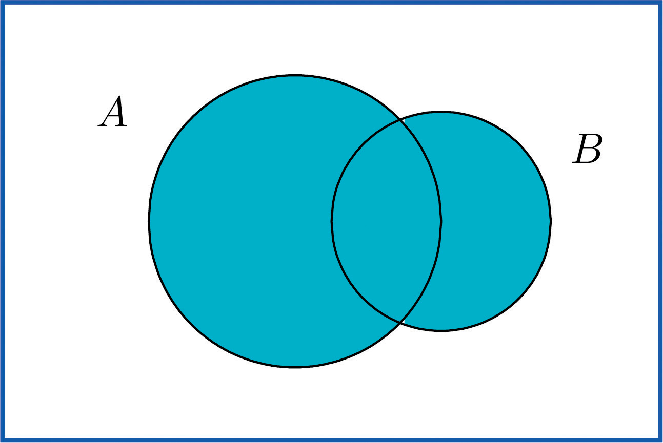
2. Intersection of Events

The intersection of events A and B, denoted A ∩ B, is the collection of all outcomes that are elements of both of the sets A and B. It corresponds to combining descriptions of the two events using the word “and.” ( A ∩ B )

The Intersection of Events A and B (A ∩ B)

EXAMPLE 12. In the experiment of rolling a single die, find the intersection E∩T of the events E : “the number rolled is even” and T : “the number rolled is greater than two.”

[ Solution ]

$S = \{1,2,3,4,5,6\}$

$E = \{2,4,6\}$ , $T = \{3,4,5,6\}$ $=> E ∩ T = \{4, 6\}$

• in prob Package : intersect()

R Source

library(prob)

# 1. Sample Space
S <- rolldie(1); S

# 2. E and E Complement
E <- subset(S, X1 %% 2 == 0); E

# 3. T and T Complement
T <- subset(S, X1 > 2); T

# 4. Intersect of E and T
intersect(E,T)

Sample Space

E

T

E ∩ T

• in Rstat Package : intersect2()

R Source

library(Rstat)

# 1. Sample Space
S <- rolldie2(1); element(S)

# 2. E and E Complement
E <- subset(S, X1 %% 2 == 0); element(E)

# 3. T and T Complement
T <- subset(S, X1 > 2); element(T)

# 4. Intersect of E and T
ET <- intersect2(E,T); element(ET)

Result

EXAMPLE 13. A single die is rolled.

1. Suppose the die is fair. Find the probability that the number rolled is both even and greater than two.

2. Suppose the die has been “loaded” so that $P(1)=1∕12$ , $P(6)=3∕12$ , and the remaining four outcomes are equally likely with one another. Now find the probability that the number rolled is both even and greater than two.

[ Solution ]

$S=\{1,2,3,4,5,6\}, A = \{2,4,6\} , B=\{3,4,5,6\}, A ∩ B =\{4, 6\}$

1. $P(A ∩ B) =P\{4, 6\} = P(4) + P(6) = 2/6 = 1/3$

2. $P(A ∩ B) =P\{4, 6\} = P(4) + P(6)$ $P(4) = ( 1 - 1/12 - 3/12) /4 = 2/12 = 1/6$ $=> P(4,6) = 1/6 + 3/12 = 5/12$

* Probability Rule for Mutually Exclusive Events

Events A and B are mutually exclusive if they have no elements in common.

Events A and B are mutually exclusive if and only if

$P(A∩B)=0$

EXAMPLE 14. In the experiment of rolling a single die, find three choices for an event $A$ so that the events $A$ and $E$: “the number rolled is even” are mutually exclusive.

[ Solution ]

Since $E=\{2,4,6\}$ and we want $A$ to have no elements in common with $E$ , any event that does not contain any even number will do. Three choices are $\{1,3,5\}$ (the complement $E^c$ , the odds), $\{1,3\}$ , and $\{5\}$ .

• Using Rstat Package

R Source

library(Rstat)

# 1. Sample Space
S <- rolldie2(1); element(S)

# 2. E
E <- subset(S, X1 %% 2 == 0); element(E)

Result

3. Union of Events

The union of events A and B, denoted $A ∪ B$ , is the collection of all outcomes that are elements of one or the other of the sets A and B, or of both of them. It corresponds to combining descriptions of the two events using the word “or.”

The Union of Events A and B : A ∪ B

EXAMPLE 15. In the experiment of rolling a single die, find the union of the events $E$ : “the number rolled is even” and $T$ : “the number rolled is greater than two.”

[ Solution ]

Since the outcomes that are in either $E=\{2,4,6\}$ or $T=\{3,4,5,6\}$ (or both) are 2, 3, 4, 5, and 6, $E∪T=\{2,3,4,5,6\}$ . Note that an outcome such as 4 that is in both sets is still listed only once (although strictly speaking it is not incorrect to list it twice).

In words the union is described by “the number rolled is even or is greater than two.” Every number between one and six except the number one is either even or is greater than two, corresponding to $E ∪ T$ given above.

• in prob Package : union()

R Source

library(prob)

# 1. Sample Space
S <- rolldie(1); S

# 2. E
E <- subset(S, X1 %% 2 == 0); E

# 3. T
T <- subset(S, X1 > 2); T

# 4. Union of E and T
union(E,T)

Sample Space

E

T

E ∪ T

• in Rstat Package : union2()

R Source

library(Rstat)

# 1. Sample Space
S <- rolldie2(1); element(S)

# 2. E
E <- subset(S, X1 %% 2 == 0); element(E)

# 3. T
T <- subset(S, X1 > 2); element(T)

# 4. Union of E and T
ET <- union2(E,T)
ET <- ET[order(ET$X1),]
element(data.frame(ET))

Result

EXAMPLE 16. A two-child family is selected at random. Let $B$ denote the event that at least one child is a boy, let $D$ denote the event that the genders of the two children differ, and let $M$ denote the event that the genders of the two children match. Find $B ∪ D$ and $B∪M$ .

[ Solution ]

A sample space for this experiment is $S=\{bb,bg,gb,gg\}$ , where the first letter denotes the gender of the firstborn child and the second letter denotes the gender of the second child. The events $B$, $D$, and $M$ are

$B=\{bb,bg,gb\}$   $D=\{bg,gb\}$   $M=\{bb,gg\}$

Each outcome in $D$ is already in $B$, so the outcomes that are in at least one or the other of the sets $B$ and $D$ is just the set $B$ itself: $B∪D=\{bb,bg,gb\}=B$ .

Every outcome in the whole sample space S is in at least one or the other of the sets $B$ and $M$, so $B∪M=\{bb,bg,gb,gg\}=S$ .

• Using prob Package

R Source

library(prob)

# 1. Sample Space
S <- data.frame(c1=c("b","b","g","g"), c2=c("b","g","b","g")); S

# 2. B, D, M
B <- subset(S, as.numeric(c1) + as.numeric(c2) < 4); B

D <- subset(S, c1 != c2); D

M <- subset(S, c1 == c2); M

# 3. B∪D and B∪M
union(B, D)

union(B, M)

Sample Space

B, D, M

B∪D and B∪M

• Using Rstat Package

R Source

library(Rstat)

# 1. Sample Space
S <- data.frame(c1=c("b","b","g","g"), c2=c("b","g","b","g")); element(S)

# 2. B, D, M
B <- subset(S, as.numeric(c1) + as.numeric(c2) < 4); element(B)
D <- subset(S, c1 != c2); element(D)
M <- subset(S, c1 == c2); element(M)

# 3. B∪D and B∪M
BuD <- union(B, D); element(BuD)
BuM <- union(B, M); element(BuM)

Result

Additive Rule of Probability

$P(A∪B)=P(A)+P(B)−P(A∩B)$

EXAMPLE 17. Two fair dice are thrown. Find the probabilities of the following events:

1. both dice show a four

2. at least one die shows a four

[ Solution ]

As was the case with tossing two identical coins, actual experience dictates that for the sample space to have equally likely outcomes we should list outcomes as if we could distinguish the two dice. We could imagine that one of them is red and the other is green. Then any outcome can be labeled as a pair of numbers as in the following display, where the first number in the pair is the number of dots on the top face of the green die and the second number in the pair is the number of dots on the top face of the red die.

11  12  13  14  15  16
21  22  23  24  25  26  
31  32  33  34  35  36
41  42  43  44  45  46
51  52  53  54  55  56
61  62  63  64  65  66

1. There are 36 equally likely outcomes, of which exactly one corresponds to two fours, so the probability of a pair of fours is 1/36.

2. From the table we can see that there are 11 pairs that correspond to the event in question: the six pairs in the fourth row (the green die shows a four) plus the additional five pairs other than the pair 44, already counted, in the fourth column (the red die is four), so the answer is 11/36. To see how the formula gives the same number, let $A_G$ denote the event that the green die is a four and let $A_R$ denote the event that the red die is a four. Then clearly by counting we get $P(A_G)=6∕36$ and $P(A_R)=6∕36$. Since $A_G∩A_R=\{44\}$ , $P(A_G∩A_R)=1∕36$ ; this is the computation in part (a), of course. Thus by the Additive Rule of Probability, $P(A_G∪A_R)=P(A_G)+P(A_R)−P(A_G−A_R)=\frac{6}{36}+\frac{6}{36}−\frac{1}{36}=\frac{11}{36}$

• Using prob Package

R Source

library(prob)

# 1. Sample Space and Number of Outcoms
S <- rolldie(2, makespace = TRUE); S

# 2. Both dice show a four
A <- subset(S, X1 == 4 & X2 == 4); A
Prob(A)

# 3. at least one die shows a four
Bc <- subset(S, X1 != 4 & X2 != 4)
B <- setdiff(S, Bc); B
Prob(B)

Sample Space

# 1.

# 2.

• Using Rstat Package

R Source

library(Rstat)

# 1. Sample Space and Number of Outcoms
S <- rolldie2(2); 
S <- S[order(S$X1, S$X2), ]
element(S, 6)

# 2. Both dice show a four
A <- subset(S, X1 == 4 & X2 == 4); element(A)
pprt(A, nrow(S))

# 3. at least one die shows a four
Bc <- subset(S, X1 != 4 & X2 != 4)
B <- setdiff2(S, Bc); element(B, 6)
pprt(B, nrow(S))

Result

EXAMPLE 18. A tutoring service specializes in preparing adults for high school equivalence tests. Among all the students seeking help from the service, 63% need help in mathematics, 34% need help in English, and 27% need help in both mathematics and English. What is the percentage of students who need help in either mathematics or English?

[ Solution ]

Imagine selecting a student at random, that is, in such a way that every student has the same chance of being selected. Let $M$denote the event “the student needs help in mathematics” and let $E$ denote the event “the student needs help in English.” The information given is that $P(M)=0.63$ , $P(E)=0.34$ , and $P(M∩E)=0.27$ . The Additive Rule of Probability gives

$P(M∪E)=P(M)+P(E)−P(M∩E)=0.63+0.34−0.27=0.70$

EXAMPLE 19. Volunteers for a disaster relief effort were classified according to both specialty ( $C$ : construction, $E$: education, $M$: medicine) and language ability ( $S$ : speaks a single language fluently, $T$ : speaks two or more languages fluently). The results are shown in the following two-way classification table:

The first row of numbers means that 12 volunteers whose specialty is construction speak a single language fluently, and 1 volunteer whose specialty is construction speaks at least two languages fluently. Similarly for the other two rows.

A volunteer is selected at random, meaning that each one has an equal chance of being chosen. Find the probability that:

1. his specialty is medicine and he speaks two or more languages;

2. either his specialty is medicine or he speaks two or more languages;

3. his specialty is something other than medicine.

[ Solution ]

When information is presented in a two-way classification table it is typically convenient to adjoin to the table the row and column totals, to produce a new table like this:

	Language Ability
Specialty	S	T	Total
C	12	1	13
E	4	3	7
M	6	2	8
Total	22	6	28

1. The probability sought is $P(M∩T)$ . The table shows that there are 2 such people, out of 28 in all, hence $P(M∩T)=2∕28≈0.07$ or about a 7% chance.

2. The probability sought is P(M∪T).P(M∪T). The third row total and the grand total in the sample give $P(M)=8∕28$ . The second column total and the grand total give $P(T)=6∕28$ . Thus using the result from part (a), $P(M∪T)=P(M)+P(T)−P(M∩T)=8/28+6/28−2/28=12/28≈0.43$

   or about a 43% chance./

3. This probability can be computed in two ways. Since the event of interest can be viewed as the event C ∪ E and the events C and E are mutually exclusive, the answer is, using the first two row totals, $P(C∪E)=P(C)+P(E)−P(C∩E)=13/28+7/28−0/28=20/28≈0.71$

   On the other hand, the event of interest can be thought of as the complement $M^c$ of $M$, hence using the value of $P(M)$ computed in part (b), $P(M^c)=1−P(M)=1−8/28=20/28≈0.71$

   as before.

EXAMPLE 20. Four fair dice are thrown. Find the probabilities of the following events:

1. $A$ = sum of four dice is greater than or equal to 15.

2. $B$ = at least one die shows a six

3. $C$ = at least one die shows a one

4. $P(A∩B), P(A∩C), P(B∩C), P(A∩B∩C)$

5. $P(A∪B), P(A∪C), P(B∪C), P(A∪B∪C)$

6. $P(A∩B^c), P(A^c∩B^c), P(A∩B∩C^c), P(A∩B^c∩C)$.

And draw a Venn Diagram.

R Source

library(Rstat)

# 0. Sample Space and Number of Outcoms
S <- rolldie2(4); N <- nrow(S)

# 1. sum of four dice is greater than or equal to 15
A <- subset(S, X1+X2+X3+X4 >= 15)
pprt(A, N)

# 2. at least one die shows a six
B <- subset(S, apply(S, 1, max) == 6)
pprt(B, N)

# 3. at least one die shows a one
C <- subset(S, apply(S, 1, min) == 1)
pprt(C, N)

# 4. Intersection of A, B, C
AB <- intersect2(A,B)
AC <- intersect2(A,C)
BC <- intersect2(B,C)
ABC <- intersect2(AB,C)
pprt(AB, N)
pprt(AC, N)
pprt(BC, N)
pprt(ABC, N)

# 5. Union of A, B, C
AuB <- union2(A,B)
AuC <- union2(A,C)
BuC <- union2(B,C)
AuBuC <- union2(AuB,C)
pprt(AuB, N)
pprt(AuC, N)
pprt(BuC, N)
pprt(AuBuC, N)

# 6.
Ac <- setdiff2(S, A); Bc <- setdiff2(S, B); Cc <- setdiff2(S, C)

ABc <- intersect2(A, Bc); pprt(ABc, N)
AcBc <- intersect2(Ac, Bc); pprt(AcBc, N)
ABCc <- intersect2(AB, Cc); pprt(ABCc, N)
ABcC <- intersect2(ABc, C); pprt(ABcC, N)

# Draw a venn diagram
# install.packages("gplots")
library(gplots)
Av <- rownames(A); Bv <- rownames(B); Cv <- rownames(C)
win.graph(7,4); par(mar=c(0,2,0,2))
venn(list(Av, Bv, Cv), showSet=T)

Result

Venn Diagram

1. 补集(Complement)

2. 交集(Intersection)

3. 互斥（Mutually Exclusive）

4. 并集(Union)