9-2. Comparison of Two Population Means: Small, Independent Samples

When one or the other of the sample sizes is small, as is often the case in practice, the Central Limit Theorem does not apply. We must then impose conditions on the population to give statistical validity to the test procedure. We will assume that both populations from which the samples are taken have a normal probability distribution and that their standard deviations are equal.

1. Confidence Intervals

When the two populations are normally distributed and have equal standard deviations, the following formula for a confidence interval for $(μ_1−μ_2)$ is valid.

$100(1−α)\%$ Confidence Interval for the Difference Between Two Population Means: Small, Independent Samples

$(\bar{x_1}−\bar{x_2})±t_{α∕2} \sqrt {s^2_p(\frac{1}{n_1}+\frac{1}{n_2})}$

where $s_p^2= \frac{(n_1−1) s_1^2 + (n_2−1)s_2^2} {n_1+n_2−2}$

The number of degrees of freedom is $df=(n_1+n_2−2).$

The samples must be independent, the populations must be normal, and the population standard deviations must be equal. “Small” samples means that either $n_1<30$ or $n_2<30.$

The quantity $s_p^2$ is called the pooled sample variance. It is a weighted average of the two estimates $s_1^2$ and $s_2^2$ of the common variance $σ_1^2=σ_2^2$ of the two populations.

EXAMPLE 4. A software company markets a new computer game with two experimental packaging designs. Design 1 is sent to 11 stores; their average sales the first month is 52 units with sample standard deviation 12 units. Design 2 is sent to 6 stores; their average sales the first month is 46 units with sample standard deviation 10 units. Construct a point estimate and a 95% confidence interval for the difference in average monthly sales between the two package designs.

[ Solution ]

• Step 1. The point estimate of $(μ_1−μ_2)$ is $(\bar{x_1}−\bar{x_2})=52−46=6$ In words, we estimate that the average monthly sales for Design 1 is 6 units more per month than the average monthly sales for Design 2.

• Step 2. To apply the formula for the confidence interval, we must find $t_{α∕2}.$ The 95% confidence level means that $α = (1 − 0.95) = 0.05$ so that $t_{α∕2}=t_{0.025}.$ From Figure 12.3 "Critical Values of ", in the row with the heading $df = (11 + 6 − 2) = 15$ we read that $t_{0.025}=2.131.$ From the formula for the pooled sample variance we compute $s_p^2= \frac{(n_1−1) s_1^2 + (n_2−1)s_2^2} {n_1+n_2−2} =\frac {(10)(12)^2+(5)(10)^2 } {15}=129.3$ Thus $(\bar{x_1}−\bar{x_2})±t_{α∕2} \sqrt {s^2_p(\frac{1}{n_1}+\frac{1}{n_2})}$ $= 6 ± (2.131) \sqrt{129.3 (\frac{1}{11} +\frac{1}{6})} ≈6±12.3$

• We are 95% confident that the difference in the population means lies in the interval $[−6.3,18.3],$ in the sense that in repeated sampling 95% of all intervals constructed from the sample data in this manner will contain $(μ_1−μ_2)$. Because the interval contains both positive and negative values the statement in the context of the problem is that we are 95% confident that the average monthly sales for Design 1 is between 18.3 units higher and 6.3 units lower than the average monthly sales for Design 2.

2. Hypothesis Testing

Testing hypotheses concerning the difference of two population means using small samples is done precisely as it is done for large samples, using the following standardized test statistic. The same conditions on the populations that were required for constructing a confidence interval for the difference of the means must also be met when hypotheses are tested.

Standardized Test Statistic for Hypothesis Tests concerning the Difference Between Two Population Means: Small, Independent Samples

$t_o = \frac{(\bar{x_1}−\bar{x_2}) -D_0 } { \sqrt {s^2_p(\frac{1}{n_1}+\frac{1}{n_2})} }$

where $s_p^2= \frac{(n_1−1) s_1^2 + (n_2−1)s_2^2} {n_1+n_2−2}$

The test statistic has Student’s t-distribution with $df=(n_1+n_2−2)$ degrees of freedom.

The samples must be independent, the populations must be normal, and the population standard deviations must be equal. “Small” samples means that either $n_1<30$ or $n_2<30$

.

EXAMPLE 5. Refer to Note 9.11 "Example 4" concerning the mean sales per month for the same computer game but sold with two package designs. Test at the 1% level of significance whether the data provide sufficient evidence to conclude that the mean sales per month of the two designs are different. Use the critical value approach.

[ Solution ]

• Step 1. The relevant hypothsis test is $H0:μ1−μ2=0 vs.  Ha:μ1−μ2≠0, @ α=0.01$

• Step 2. Since the samples are independent and at least one is less than 30 the test statistic is $t_o = \frac{(\bar{x_1}−\bar{x_2}) -D_0 } { \sqrt {s^2_p(\frac{1}{n_1}+\frac{1}{n_2})} }$

  which has Student’s t-distribution with $df=(11+6−2)=15$ degrees of freedom.

• Step 3. Inserting the data and the value $D_0=0$ into the formula for the test statistic gives $t_o = \frac{(\bar{x_1}−\bar{x_2}) -D_0 } { \sqrt {s^2_p(\frac{1}{n_1}+\frac{1}{n_2})} } = \frac {(52−46)−0}{129.3 (\frac{1}{11}+\frac{1}{6})} ≈ 1.040$

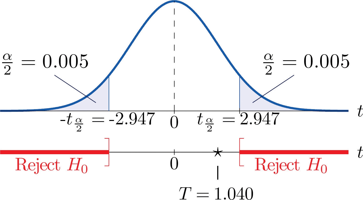
• Step 4. Since the symbol in $H_a$ is “ $≠$ ” this is a two-tailed test, so there are two critical values, $±t_{α∕2}=±t_{0.005}.$ From the row in Figure 12.3 "Critical Values of " with the heading $df=15$ we read off $t_{0.005}=2.947.$ The rejection region is $(−∞,−2.947]∪[2.947,∞).$

• Step 5. As shown in Figure 9.4 "Rejection Region and Test Statistic for " the test statistic does not fall in the rejection region. The decision is not to reject $H_0$ .

• In the context of the problem our conclusion is:

  The data do not provide sufficient evidence, at the 1% level of significance, to conclude that the mean sales per month of the two designs are different.

Figure 9.4 Rejection Region and Test Statistic for Note 9.13 "Example 5"

EXAMPLE 6. Perform the test of Note 9.13 "Example 5" using the p-value approach.

[ Solution ]

• Step 4. Because the test is two-tailed the observed significance or p-value of the test is the double of the area of the right tail of Student’s t-distribution, with 15 degrees of freedom, that is cut off by the test statistic T = 1.040. We can only approximate this number. Looking in the row of Figure 12.3 "Critical Values of " headed $df=15$ , the number 1.040 is between the numbers 0.866 and 1.341, corresponding to $t_{0.200}$ and $t_{0.100}.$

  The area cut off by t = 0.866 is 0.200 and the area cut off by t = 1.341 is 0.100. Since 1.040 is between 0.866 and 1.341 the area it cuts off is between 0.200 and 0.100. Thus the p-value (since the area must be doubled) is between 0.400 and 0.200.

• Step 5. Since $p>0.200>0.01, p>α,$ so the decision is not to reject the null hypothesis:

  The data do not provide sufficient evidence, at the 1% level of significance, to conclude that the mean sales per month of the two designs are different.